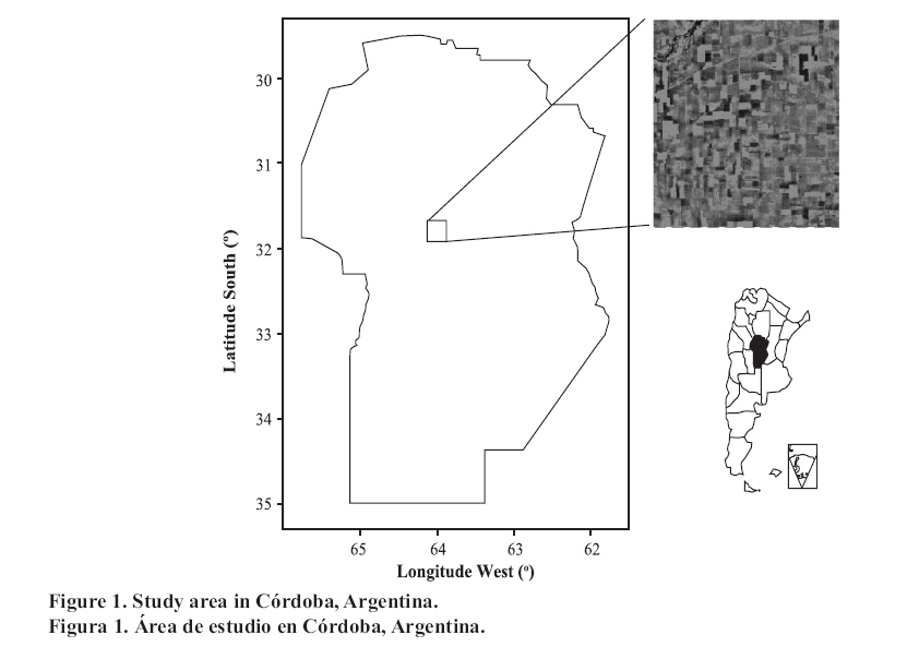
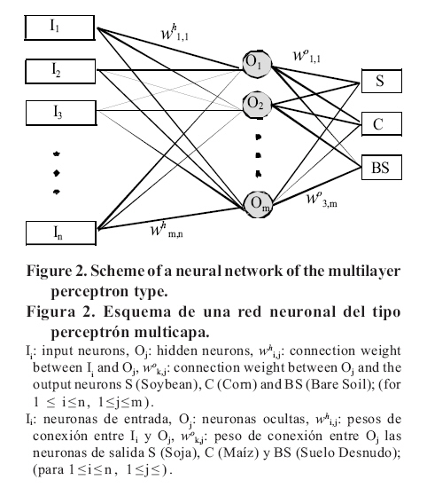
Agricultura Técnica, Vol. 67, No. 4, Oct-Dec, 2007 pp. 414-421

Research

NEURAL NETWORK MODELS FOR LAND COVER CLASSIFICATION FROM SATELLITE IMAGES

Modelos de redes neuronales para la clasificación de cobertura del suelo a partir de imágenes satelitales¹

Mónica Bocco[1]*,Gustavo Ovando¹, Silvina Sayago¹ and Enrique Willington¹

[1] Universidad Nacional de Córdoba, Facultad de Ciencias Agropecuarias, CC 509 (5000), Córdoba, Argentina. E-mail: mbocco@agro.uncor.edu   * Corresponding author.

Received: 26 February 2007.                            
Accepted: 23 March 2007.

Code Number: at07049

ABSTRACT 

Land cover data represent environmental information for a variety of scientific and policy applications, so its classification from satellite images is important. Since neural networks (NN) do not require a hypothesis about data distribution, they are valuable tools to classify satellite images. The objectives of this work were to develop NN models to classify land cover data from information from satellite images and to evaluate them when different input variables are used. MODIS-MYD13Q1 satellite images and data of 85 plots in Córdoba, Argentina, were used. Five NN models of multi-layer feed-forward perceptron were designed. Four of these received NDVI (Normalized Difference Vegetation Index), EVI (Enhanced Vegetation Index), red (RED) and near infrared (NIR) reflectance values as input patterns, respectively. The fifth NN had RED and NIR reflectances as input values. By comparing the information taken in the field and the classification made during the validation phase, it can be concluded that all models presented good performance in the classification. The model that shows better behavior is the one that jointly considers RED and NIR reflectance as input; this model shows an overall classification accuracy of 93% and an excellent Kappa statistic. The networks constructed with NDVI and EVI values have a similar behavior (86 and 83% accuracy, respectively). The Kappa statistics correspond to the categories of very good and good, respectively. The networks including only RED or NIR reflectance values get the lowest accuracy results (76 and 81%, respectively) and Kappa values within fair and good ranks, respectively.

Keywords: modeling, back-propagation neural networks, remote sensing, crops-bare soil.

RESUMEN 

Los datos de cobertura de suelo representan información ambiental clave para aplicaciones científicas y políticas, por esto su clasificación a partir de imágenes satelitales es importante. Las redes neuronales (NN) constituyen una herramienta valiosa para clasificar imágenes satelitales pues no requieren hipótesis sobre la distribución de los datos. Los objetivos de este trabajo fueron desarrollar modelos de NN para clasificar datos de cobertura de suelo a partir de información proveniente de imágenes satelitales y evaluarlos cuando se utilizan diferentes variables de entrada. Se utilizaron imágenes satelitales MODIS-MYD13Q1 y datos de 85 parcelas en Córdoba (Argentina). Se diseñaron cinco NN del tipo perceptrón multicapa feed-forward. Cuatro de ellas recibieron como patrones de entrada valores de NDVI (Normalized Difference Vegetation Index), EVI (Enhanced Vegetation Index), de reflectancias en la bandas roja (RED) y en infrarroja cercana (NIR), respectivamente. La quinta NN tuvo como valores de entrada las reflectancias RED y NIR. La validación, permitió concluir que todos los modelos presentan un buen desempeño. El modelo que muestra mejor comportamiento es aquel que considera conjuntamente valores de reflectancias RED y NIR, cuya precisión en la clasificación es del 93% con un estadístico Kappa excelente. Las redes construidas individualmente a partir de valores de NDVI y EVI tienen un comportamiento similar (86 y 83% de exactitud, respectivamente), con estadísticos Kappa  muy bueno y bueno, respectivamente. Las NN que incluyen sólo valores de RED o NIR presentaron los menores porcentajes de exactitud (76 y 81%, respectivamente) con índices Kappa regular y bueno, respectivamente.

Palabras clave: modelación, redes neuronales backpropagation, teledetección, cultivos-suelo desnudo.

INTRODUCTION

Land cover data are among the most important and universally used terrestrial data sets and represent key environmental information for a variety of scientific and policy applications (Cihlar, 2000; De Fries and Belward, 2000).

The extraction of useful information from satellite images, by means of classification, is one of the most important technical problems of remote sensing. The objective of remote sensing is the determination of characteristics and phenomena that take place on the earth’s surface. Through its spectral signature, remote sensing studies the temporal, spatial and spectral variations of earth’s surface (Chuvieco, 2000).

Classifications are generally made from images generated by LANDSAT TM (Rizzi and Rudorff, 2005); in Argentina, Guerschman et al. (2003) used multi-temporal LANDSAT TM data from the same growing season for the classification of land cover types in the south-western portion of the Pampas.

High-resolution data from sensors such as LANDSAT TM would be more suitable in areas where the field sizes are small. However, temporal frequency and cloud cover limit the retrieval of crop biophysical parameters that are rapidly changing during the season. The spatial and temporal resolution of MODIS data offer, in turn, a great potential for obtaining these biophysical parameters (Doraiswamy et al., 2005). In this sense, Reed et al. (1996) proposed using a fine temporal resolution in order to classify great areas and, thus, identify the changes that take place in the spatial and temporal scales.

As regards spectral resolution, one of the earliest digital remote-sensing analysis procedures developed to identify the vegetation contribution in an image was the ratio vegetation index, created by dividing near infrared reflectance (NIR) by red reflectance (RED). The basis of this relationship is the strong red light absorption (low reflectance) by chlorophyll and the low absorption (high reflectance and transmittance) in the NIR by green leaves. Dense green vegetation has a high ratio while soil has a low value, thus yielding a contrast between the two surfaces (Shanahan et al., 2001). Spectral reflectance increases with wavelength and is a function of soil moisture (Stark et al., 2000).

NIR reflectance is different in each species due to its dependence on factors such as architecture of the canopy, cell structure and leaf inclination. Jackson and Pinter (1986) found that an erectophile canopy generally disperses more radiation in the lower layers than does a planophile canopy, consequently minimizing NIR reflectance. On the other hand, reflectance in the visible range is less specific on the species since it is mainly influenced by pigment content and composition (Gitelson et al., 2002).

At present, the most used vegetation index is the Normalized Difference Vegetation Index (NDVI = (NIR-RED)/(NIR+RED)), the reason being that it employs basic spectral bands available in practically all remote sensing systems and is computationally very efficient (Walthall et al., 2004). Among the disadvantages of the NDVI, the following can be mentioned: the nonlinearity of ratio-based indexes, the influence of the atmosphere, scaling problems, asymptotic (saturated) signals over high biomass conditions and sensitivity to background variations (Huete et al., 2002).

In order to overcome the aforementioned disadvantages, new indexes have been developed to compensate  for both the effect of the atmosphere (Kaufman and Tanré, 1996) and soil (Huete, 1988), particularly the 'enhanced' vegetation index (EVI) with improved sensitivity in high biomass regions and improved vegetation monitoring through a de-coupling of the canopy background signal and a reduction in atmospheric influences (Liu and Huete, 1995; Huete et al., 1997).

There are different algorithms used to classify remote sensing images. The most often used of these, such as the maximum likelihood algorithm, require data with normal distribution. Among the algorithms that do not hypothesize on data distribution are the k nearest neighbours and neural networks (NN). (Walthall et al., 2004; Mas, 2005).  In this work we use NN.

Artificial NN can be used to develop empirically based agricultural models. The NN structure is based on the human brain’s biological neural processes. Interrelationships of correlated variables that symbolically represent the interconnected processing neurons or nodes of the human brain are used to develop models (Kaul et al., 2005). Neural networks are a structure of neurons joined by nodes that transmit information to other neurons, which give a result through mathematical functions. In general, an NN requires three layers: the input, hidden, and output layers. The input and output layers contain nodes that correspond to input and output variables, respectively (Hilera and Martínez, 2000).

The NN learn from the existing information through a training process by which their parameters are adjusted so as to provide an approximate output close to the desired one. Data move between layers across weighted connections. The number of hidden nodes determines the number of connections between inputs and outputs and it may vary depending on the specific problem under study. During the learning phase, a transfer function is applied through a series of iterations, so that the predicted values are compared with the observed values. The training finishes when an acceptably low error for all the learning patterns is reached. Once the network converges, an approximate function is developed and utilized for future predictions. In this way, the NN acquires the capacity to estimate answers from the same phenomenon. Finally, the trained network is then tested with an independent data set.

Crop yield estimation is a strategic regional datum and it constitutes valuable information used to determine the possible exportable surplus and to plan storage and transport. Soybean (Glycine max L. Merr.) is, at the moment, the most important crop in Argentina in relation to the sown surface (15 329 000 ha in 2005-2006 (SAGPyA, 2006) and to the economic yield obtained by farmers. Regarding corn (Zea mays L.), Córdoba is the second producer of this crop in Argentina with an approximate sown surface of 794 100 ha in the 2005-2006 crop year, according to estimations made by the Secretaría de Agricultura, Ganadería y Alimentos from Córdoba Province (SAGyA, 2006). Sown surface and yield estimation data are obtained from censuses and surveys.

The main objective of this research was to develop neural network models capable of classifying land cover (soybean, corn, bare soil) using information taken from MODIS satellite images and evaluating behavior of those networks and classification errors by using different input variables.

MATERIALS AND METHODS 

Study area. The study area was located in the central plains of Córdoba Province, Argentina (Figure 1 ), in the sub-region known as “Pampa Alta” ( aprox. 32º S; 64º W), which presents a slightly undulating relief of hills developed on loessic material, of silt loam texture with a slight slope to the east. Soils in this area are classified as Entic and Typic Haplustol. The average annual rainfall is approximately 800 mm, concentrated in summer, thus it belongs to a monzonic regime (INTA, 2003). The climate in the study area is classified as dry sub-humid (Mather, 1965).

The areas for agricultural production have mainly summer crops (soybean and corn) and, to a lesser degree, winter cereals (wheat, Triticum aestivum L.). Sowing of crops responds to climatic conditions, particularly rainfall distribution.

Ground data. For the survey, data of 85 plots were collected. The plots should have an area larger than 50 ha to adjust to the resolution of the MODIS sensor; 13% of the plots presented bare soil, 63.5% were cultivated with soybean and 23.5% with corn. Field data acquisition was carried out at the end of December 2005, when soybean crop had one to eight open trifoliate leaves and corn had from six open leaves to silking.

Satellite data. Three images from AQUA satellite were used for the period from December 3, 2005 to January 16, 2006. These came from the MODerate-resolution Imaging Spectroradiometer (MODIS-MYD13Q1/Aqua 16-Day integrated L3 Global 250 m SIN Grid) and were obtained by the Land Processes Distributed Active Archive Center (LPDAAC)–US Geological Center (USGS) for Earth Resources Observation and Science (EROS) Data Center, located in Sioux Falls, South Dakota, USA.

This time period was considered since both cultures have different thermal requirements, and thus, different sowing dates (first corn and then soybean). This time interval allowed the discrimination of corn in reproductive stages from soybean in vegetative stages.

NDVI daily images in a continuous time series do not always describe the condition of vegetation precisely during the growing season, since contamination by clouds decreases the vegetation index value. Consequently, the solution is to retain a high temporal resolution uncovering and removing cloudy pixels from daily images, thus creating NDVI composite images of 10 to 15 days only, with data taken during non-cloudy days (Báez-González et al., 2002).

The MYD13Q1 product presents NDVI and EVI vegetation indexes which are used as input. The vegetation index algorithms are produced globally for the whole earth. The two vegetation indexes complement each other in global vegetation studies and improve upon the extraction of canopy biophysical parameters. A new compositing scheme that reduces angular, sun-target-sensor variations with an option of using Bidirectional Reflectance Distribution Function models is employed. The grid vegetation indexes include quality assurance flags with statistical data that indicate the quality of the vegetation index product and input data.

The MYD13Q1 product also presents reflectance values in blue (459-479 nm), red (620-670 nm), near infrared (NIR, 841-876 nm) and medium infrared (MIR, 1230-1250 nm).

Neural networks. Five NN models of the multilayer feed-forward perceptron type were designed. All of them included three layers of neurons: input, hidden and output layer (Figure 2 ). Models M1 to M4 received the NDVI, EVI, RED, NIR values respectively as input patterns. Each of them were built with three neurons in the input layer (I), corresponding to three images used. The M5 model was built using six neurons, which corresponded to RED and NIR values in the input layer. For all models, the data entered belonged to images of the whole time series utilized. In each model, the same number of neurons was utilized in the hidden layer (H) as in the input layer.

This decision was made after comparing the results of each model, when the hidden neuron number varied between 50 to 200% from total input neuron number. When the neuron number in the hidden layer was lower than the number of neurons in the input layer, the overall accuracy classification was poor, while using a large number of neurons in the hidden layer did not yield a better classification.

The hidden neuron layer produced an output using a non-linear activation function (hyperbolic tangent) to the weighted sum of the input values multiplied by the weights of the connections between neurons:

where Tanh = hyperbolic tangent, exp (x) = exponential function.

The output layer (O) produced the result utilizing the same procedures used in the hidden layer; in this case, the output layer was constituted by three neurons that corresponded to the classes describing the presence of soybean, corn or bare soil.

Classification and evaluation processes. Network learning was carried out using the back-propagation algorithm, which propagates the error back from the output layer to the input layer. This algorithm allows weight adaptation, resulting in reduced errors.

The steps that demonstrate the training algorithm of the proposed networks are described according to Bocco et al. (2006).

To accelerate the learning process, a learning rate equal to 1 was included, and to correct the direction of the error, a moment term equal to 0.7 was used in the output and hidden neurons.

In the learning phase of the designed net, a thousand repetitions were made to ensure that the minimum square error was acceptably low.

For the learning process, 43 patterns of data were used. The data number of each pattern was formed by the values of the input variables of each of three images used. The remaining 42 patterns were employed for the validation process.

For each one of the classifications from the models, a contingency matrix was generated and the overall accuracy, the Kappa statistic and the producer’s and user’s accuracy for each class were calculated. The overall accuracy was calculated through the plot ratio correctly classified (i.e., the sum of the diagonal axes) divided by the total number included in the evaluation process. The Kappa statistic is an alternative measure of classification accuracy that subtracts the effect from random accuracy. Kappa quantifies how much better a particular classification is in comparison to a random classification. Monserud and Leemans (1992) suggested the use of a subjective scale where Kappa values < 40% are poor, 40-55% fair, 55-70% good, 70-85% very good and > 85% excellent.

For individual classes, two accuracies can be calculated: 1) the producer’s accuracy is a measure of omission error and indicates the percentage of pixels of a given land cover type that are correctly classified, and 2) the user’s accuracy is a measure of the commission error and indicates the probability that a pixel classified into a given class actually represents that class on the ground.

RESULTS AND DISCUSSIONS 

All models presented good performance in land cover estimation, which can be observed by comparing the obtained error in the validation phase of the different proposed models. The accuracy values and Kappa statistic percentages shown in Table 1 were calculated for each model.

Table 1. Overall, producer and user accuracies and Kappa statistic for the models performed with different combinations of input data.

Tabla 1. Precisión total, del productor y del usuario y estadístico Kappa, para los modelos realizados con distintas combinaciones de los datos de entrada.

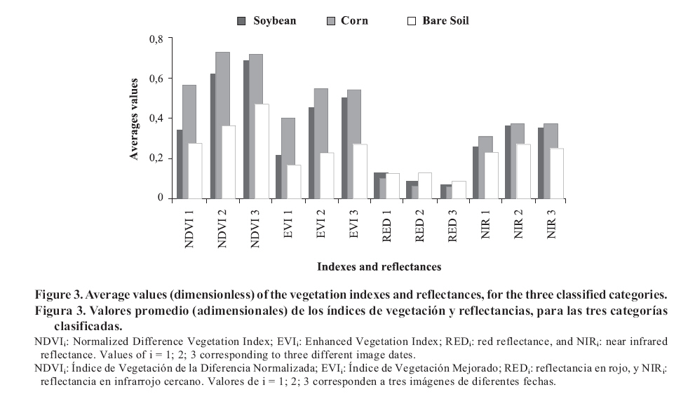
Input data for model: M1: Normalized Difference Vegetation Index; M2: Enhanced Vegetation Index; M3: red reflectance; M4. near infrared reflectance; M5: red and near infrared reflectances.
Datos de entrada para el modelo: M1: Índice de Vegetación de la Diferencia Normalizada; M2: Índice de Vegetación Mejorado; M3: reflectancia en rojo; M4: reflectancia en el infrarrojo cercano; M5: reflectancias en rojo e infrarrojo cercano.

The results in Table 1 show that the networks constructed with NDVI and EVI (M1 and M2) values have a similar behavior, which is reflected by totally similar accuracy values. The Kappa statistic of the NDVI based model corresponds to the very good category, while the index of M2 corresponds to the good category. M2 presents differences in the accuracy values (producer/user) for corn.

These differences could occur because M2 has an inferior capacity to classify corn and because the probability to randomly classify a plot of corn almost doubles the probability of classifying it as bare soil.

The networks including only RED and NIR reflectance values (M3 and M4) get the smallest global accuracy percentages (76.2 and 81.0%, respectively) and Kappa values as results, which can be considered within the fair and good ranks, respectively. For soybean, both models keep high accuracy values (producer/user).

The low accuracy value observed in bare soil, for M3, could be explained by the small number of plots in this category, but it demonstrates that networks do not identify radiometric differences between soil, and corn and soybean. In NIR, in contrast, reflectance is notably higher for bare soil in comparison to vegetation as expressed by Shanahan et al. (2001).

The difference between the vegetation indexes, RED and NIR average values for all plots and for the three classified categories can also be observed in Figure 3 , in which the sub index of each variable refers to each of the images used in the time series.

The designed network that jointly includes RED and NIR values (M5) as input variables showed the highest results in statistic validation. The total accuracy value reaches 93% approximately, with values for each class in the interval of 80 to 100%, and with an excellent Kappa statistic. From this first evaluation, it can be stated that, if the information is available, the utilization of the two reflectance values is the best combination to estimate land cover.

Accuracy values that resulted from model application are similar and/or superior to those values presented by other authors, which demonstrates that the methodology is suitable for land cover classification.

Aitkenhead and Wright (2004), who classified urban areas, crops in general and bare soil, used neural networks in a LANDSAT TM image and obtained a 60% accuracy value for commercial urban areas, 100% for water and forests, 90% for bare soil and 95% for undifferentiated crops.

In addition, when classifying NDVI multi-temporal images coming from MODIS, Wardlow and Egbert (2005) discovered an accuracy of 82% for soybean, 88.7% for corn and 78.2% for sorghum (Sorghum vulgare L.), thus they obtained a general accuracy value of 84% in Kansas State, USA, using decision trees. These values are always maintained below the results that neural networks present for the same input variable (M1).

For southern Mexico, Mas (2005) carried out a classification using neural networks in the following categories: jungle, mangrove swamp, tular, agriculture and grassland, water and urban areas. Classification from a unique image, which included five spectral bands of LANDSAT ETM, reached a global reliability of 74% (67% without taking into account the category “water”).

For Argentina, in the flooding and Southern Pampa, Guerschman et al. (2003) carried out a land cover classification for these categories: corn, sunflower (Helianthus annuus L.), soybean, sorghum, wheat, oat (Avena sativa L.) and pastures, using four LANDSTAT TM images and the maximum likelihood decision rule. The results of Kappa statistics obtained when the classification was carried out from all satellite bands were 54.7 and 50% only for NDVI. These percentages are inferior to those obtained by the models presented here.

As regards producer’s accuracy for soybean and corn, their values are 74 and 65% respectively, while the values that neural networks present for these crops are 93 and 90% respectively. User’s accuracy values were 83 and 23% for soybean and corn, respectively, while these values reached approximately 96 and 82% respectively for M5.

CONCLUSIONS 

The modeling process that uses neural networks is effective to estimate land cover from satellite images, even using a limited number of data (spectral values).

The model that shows the best behavior to classify land cover is the one that considers the reflectances in the red and infrared spectrum input values, reaching a classification accuracy of 93% approximately and an excellent Kappa statistic.

All the models designed classify soybean with similar exactitude, but show differences in the classification accuracy of corn and bare soil.

LITERATURE CITED 

• Aitkenhead, M.J., and G.G. Wright. 2004. Mapping land use in NE Scotland with neural networks from remote sensing imagery. 11 p. In Remote Sensing and Photogrammetry Society Annual Conference, Aberdeen. 6-7 September 2004. The Macaulay Institute, Craigiebuckler, UK Workshop Output. [On line] Available at http://www.macaulay.ac.uk/workshop/remotesensing2004/MA_Full_paper.pdf. Accessed September 25, 2006.
• Báez-González, A.D., P. Chen, M. Tiscareño-López, and R. Srinivasan. 2002. Using satellite and field data with crop growth modeling to monitor and estimate corn yield in Mexico. Crop Sci. 42:1943-1949.
• Bocco, M., G. Ovando, and S. Sayago. 2006. Development and evaluation of neural network models to estimate daily solar radiation at Córdoba, Argentina. Pesq. Agropec. Bras. 41:179-184.
• Cihlar, J. 2000. Land cover mapping of large areas from satellites: status and research priorities. Int. J. Remote Sens. 21:1093-1114.
• Chuvieco, E. 2000. Fundamentos de la teledetección espacial. 558 p. 3ª ed. Ed. Rialp, Madrid, España.
• De Fries, R.S., and A.S. Belward. 2000. Global and regional land cover characterization from satellite data: an introduction to the special issue. Int. J. Remote Sens. 21:1083-1092.
• Doraiswamy, P.C., T.R. Sinclair, S. Hollinger, B. Akhmedov, A. Stern, and J. Prueger. 2005. Application of MODIS derived parameters for regional crop yield assessment. Remote Sens. Environ. 97:192-202.
• Gitelson, A.A., Y.J. Kaufman, R. Stark, and D. Rundquist. 2002. Novel algorithms for remote estimation of vegetation fraction. Remote Sens. Environ. 80:76-87.
• Guerschman, J.P., J.M. Paruelo, C. Di Bella, M.C. Giallorenzi, and F. Pacin. 2003. Land cover classification in the Argentine Pampas using multi-temporal Landsat TM data. Int. J. Remote Sens. 24:3381-3402.
• Hilera González, J.R., y V.J. Martínez Hernando. 2000. Redes neuronales artificiales: fundamentos modelos y aplicaciones. 390 p. Alfaomega Ra-Ma, Madrid, España.
• Huete, A.R. 1988. A soil-adjusted vegetation index (SAVI). Remote Sens.Environ. 25:295-309.
• Huete, A.R., H.Q. Liu, K. Batchily, and W.J.D. Van Leeuwen. 1997. A comparison of vegetation indices over a global set of TM images for EOS-MODIS. Remote Sens. Environ. 59:440–451.
• Huete, A.R., K. Didan, T. Miura, E.P. Rodríguez, X. Gao, and L.G. Ferreira. 2002. Overview of the radiometric and biophysical performance of the MODIS vegetation indices. Remote Sens. Environ. 83:195-213.
• INTA. 2003. Recursos Naturales de la Provincia de Córdoba. Los Suelos. 567 p. Agencia Córdoba D.A.C. y T. SEM-Instituto Nacional de Tecnología Agropecuaria (INTA), Córdoba, Argentina.
• Jackson, R.D., and P.J. Pinter Jr. 1986. Spectral response of architecturally different wheat canopies. Remote Sens. Environ. 20:43-56.
• Kaufman, Y.J., and D. Tanré. 1996. Direct and indirect methods for correcting the aerosol effect on remote sensing. Remote Sens. Environ. 55:65-79.
• Kaul, M., R. Hill, and C. Walthall. 2005. Artificial neural networks for corn and soybean yield prediction. Agric. Syst. 85:1-18.
• Liu, H.Q., and A. Huete. 1995. A feedback based modification of the NDVI to minimize canopy background and atmospheric noise. IEEE Trans. Geosci. Remote Sens. 33:457-465.
• Mas, J.F. 2005. Un método para combinar datos espectrales e información auxiliar en una red artificial neuronal p. 3543-3549. In Anais XII Simpósio Brasileiro de Sensoriamento Remoto, Goiânia, Brasil. 16-21 abril 2005. Disponible en http://marte.dpi.inpe.br/col/ltid.inpe.br/sbsr/2004/11.16.18.07/doc/3543.pdf. Leído el 25 de septiembre de 2006.
• Mather, J.R. 1965. Average climatic water balance data of the continents. Part VIII. South America. Publications in Climatology. Volume XVIII. Number 2. Laboratory of Climatology, Centerton, New Jersey, USA.
• Monserud, R.A., and R. Leemans. 1992. Comparing global vegetation maps with the Kappa statistic. Ecol. Model. 62:275-293.
• Reed, B.C., T.R. Loveland, and L.L. Tieszen. 1996. An approach for using AVHRR data to monitor U.S. Great Plains grasslands. Geocarto International 11:13-22.
• Rizzi, R., e B.F.T. Rudorff. 2005. Estimativa da área de soja no Rio Grande do Sul por meio de imagens Landsat. Revista Brasileira de Cartografia 57:226-234.
• SAGyA. 2006. Secretaría de Agricultura, Ganadería y Alimentos de la provincia de Córdoba, Argentina. Departamento de cultivos extensivos, estadísticas. Available in http://www.cba.gov.ar/vercanal.jsp?idCanal=4350. Accessed September 25, 2006.
• Shanahan, J.F., J.S. Schepers, D.D. Francis, G.E. Varvel, W.W. Wilhelm, J.M. Tringe, et al. 2001. Use of remote sensing imagery to estimate corn grain yield. Agron. J. 95:583-589.
• Stark, R., A.A. Gitelson, U. Grits, D. Rundquist, and Y. Kaufman. 2000. New technique for remote estimation of vegetation fraction: principles, algorithms and validation. Aspect Appl. Biol. 60:241-246.
• Wardlow, B.D., and S.L. Egbert. 2005. State-level crop mapping in the U.S. Central Great Plains agroecosystem using MODIS 250-meter NDVI data. 12 p. In PECORA 16 “Global Priorities in Land Remote Sensing”, Sioux Falls, South Dakota. 23-27 October 2005. Available at http://edc2.usgs.gov/pecora16/pecora_abstracts2.asp?id=104366  Accessed September 25, 2006.
• Walthall, C., W. Dulaney, M. Anderson, J. Norman, H. Fang, and S. Liang. 2004. A comparison of empirical and neural network approaches for estimating corn and soybean leaf area index from Landsat ETM+ imagery. Remote Sens. Environ. 92:465-474.

Copyright 2007 - Instituto de Investigaciones Agropecuarias, INIA (Chile).