Chilean Journal of Agricultural Research Instituto de Investigaciones Agropecuarias, INIA ISSN: 0718-5820 EISSN: 0718-5839 Vol. 68, Num. 1, 2008, pp. 56-68

Chilean Journal of Agricultural Research (formerly Agricultura Técnica), Vol. 68, No. 1, Jan-March, 2007 pp. 56-68

Research

Evaluation of The Impact of Climatic Change on the Economic Value of Land in Agricultural Systems in Chile

Evaluación del Impacto del Cambio Climático Sobre el Valor Económico de la Tierra en Sistemas Agrícolas de Chile

Jorge González U.[1]*, and Roberto Velasco H.¹

This paper is based on the SACPR project on the impact of global warming in Latin America, carried out by Yale University (USA), IICA/PROCISUR, the World Bank, INIA Chile, EMBRAPA Brazil, INTA Argentina, INIA Uruguay, INIAP Ecuador, INIA Venezuela, and CORPOICA Colombia.
[1] Instituto de Investigaciones Agropecuarias, Quilamapu Regional Research Center, Casilla 426, Chillán, Chile. E-mail: jgonzale@inia.cl * Corresponding author.

Received: 22 January 2007.
Accepted: 31 May 2007.

Code Number: cj08006

ABSTRACT

Climatic change will affect crop yields and management. By the year 2050, the mean temperature could increase by 1.5 ºC; and by the year 2100 between 1.0 to 3.5 ºC. There are few studies on this subject in Chile. At the international level, estimated climatic changes in temperate and tropical zones could negatively affect wheat (Triticum vulgare L.) and corn (Zea mays L.) production, as examples. The objective of this study was to determine the relationship between agricultural systems and climatic change by using the Ricardian Method. Specific objectives were to evaluate and quantify the relationship of climatic variables (precipitation and temperature) with economic variables under several realities of farms, to simulate the impact of scenarios of climatic change, to propose general orientations of adaptation and to evaluate the Ricardian Method with Chilean data. Economic and productive information from farmers belonging to Technological Transfer Groups (GTT)of the Agricultural Research Institute (INIA) was collected. The Ricardian Method explained 37.6% of land value variation. The highest values were in areas with moderate temperatures and precipitation. Temperature had a lower relationship to land value than precipitation. Under specific conditions (type of producer, irrigation, extension)  were detected behaviors that require further analysis. Upon simulating change of temperature and precipitation, the negative impacts on land value tended to be of lower magnitude than in other warmer regions. A tendency was observed for increased temperature to be beneficial, and a neutral to positive effect with less precipitation. The outputs could initially guide specific strategies of adaptation and mitigation.

Key words: climate change, Ricardian method, land productivity, land value, policy of adaptation

RESUMEN

El cambio climático afectará los rendimientos y manejo de los cultivos agrícolas. Se estima que al año 2050 la temperatura media aumentaría 1,5 ºC, y al 2100 entre 1,0 y 3,5 ºC. En Chile existen pocos estudios sobre el tema. Internacionalmente se estiman cambios en zonas templadas y tropicales que afectarían negativamente, por ejemplo, al cultivo de trigo (Triticum vulgare L.) y maíz (Zea mays L.). El objetivo de este estudio fue determinar la relación entre sistemas agropecuarios y cambio climático aplicando el Método Ricardiano. Los objetivos específicos fueron evaluar y cuantificar la relación de las variables climáticas (precipitación y temperatura) con variables económicas bajo diferentes realidades prediales, simular impacto de escenarios de cambio climático, proponer orientaciones generales de adaptación y evaluar el Método Ricardiano con datos chilenos. Se colectó información económica-productiva de agricultores de los Grupos de Transferencia Tecnológica (GTT) del Instituto de Investigaciones Agropecuarias (INIA). El Método Ricardiano explicó el 37,6% de la variación del valor del suelo. Los mayores valores estaban en localidades con temperaturas y precipitaciones moderadas. La temperatura presentó menor relación con el valor del suelo que la precipitación. Bajo algunas condiciones (tipo de productor, riego, capacitación) se detectaron comportamientos que requieren mayor análisis. Al simular cambios de temperatura y precipitación los impactos negativos en el valor del suelo tienden a ser menores que en regiones cálidas. Incluso se observó una leve tendencia a ser beneficiosos al aumentar la temperatura, y neutros a positivos con precipitaciones menores. Los resultados pueden orientar inicialmente estrategias específicas de adaptación y mitigación.    

Palabras clave:cambio climático, Método Ricardiano, productividad, valor tierra, políticas de mitigación.

INTRODUCTION

Agriculture depends on climatic factors such as temperature and precipitation. Although there is evidence of global warming and that this phenomenon will affect agricultural productivity, there is little quantified information on the potential impact.  Nevertheless, studies such as the one of Jones et al. (1997), suggest that the direct effects will be on crop yields and crop management, and that the indirect effects will influence aspects of technical economic analysis of the implementation of new policies and strategies. With regard to the former, it is difficult to anticipate impacts, given that the responses of agricultural producers and the results on crop yields, in the context of technological changes, are uncertain.  The European Commission has stated that by the year 2050, the average temperature of the planet will have increased by 1.5 ºC, and that by the year 2100, it will have increased by between 1.0 and 3.5ºC (European Commission, 1997).

There are practically no studies in Chile that provide data or quantifiable relationships among climatic factors, productive characteristics and economic values of agricultural systems, that would allow for developing or applying models to orient strategies of response to climatic change. The scenario could be very complex if we consider that the agricultural sector generates on the order of 6.5% of Gross National Product (ODEPA, 2006), employs 11.6% of the labor force (INE, 2006), and generates 18% of national exports (Banco Central, 2006).

There are international studies that estimate possible impacts of climatic change (Rosenzweig and Parry, 1994; Rosenzweig and Iglesias, 1994; Jones et al., 1997; CGIAR, 1998) which, in general terms, have described eventual significant changes in temperate and tropical zones in the African sub-Sahara.  Studies have also been done in Brazil (Siqueira et al., 1994; Sanghi et al., 1997; Alves and Evenson, 1996; Mendelsohn, 1996) that suggest, among other aspects, the eventual fall in the productivity of wheat and corn and the tendency toward more negative impacts in the northeast of the country. 

This study is part of a project supported by the Department of Forestry and Environmental Studies of Yale University, USA, and co-financed by the World Bank, in which IICA/PROCISUR and the national agricultural research institutes of the southern cone countries participated.  The objective was to generate preliminary information on the effect of global climatic change on agricultural systems at the respective national levels, and to quantify the relationship of temperature and precipitation to some economic characteristics of agricultural systems. Given that the effects of climatic change are cumulative and of the medium and long term, it is hoped to make a contribution in generating the basis for public agricultural policies on this theme and strategies of productive and technological adaptation by this sector.                                                                                                                        

MATERIALS AND METHODS

The Ricardian Method

The fundamental supposition of the Ricardian Method (RM) is that the agricultural producer seeks to maximize economic utility, making decisions according to market prices and other factors, such as climatic variables. The fundamental development of RM was by Mendelson et al. (1994) and it has been applied in the United States (Mendelsohn et al., 1994; Mendelsohn, 1996; 1999; 2001), Brazil (Mendelsohn et al., 2001), India (Dinar et al., 1998; Kumar and Parikh, 2001), Great Britain (Maddison, 2000) and Canada (Reinsborough, 2003). The RM postulates the relationship between productivity and climate (Mendelsohn et al., 1994), numerically estimating the impacts of climatic variables on agricultural variables. The RM incorporates productivity, using economic proxy variables, such as rural incomes, or, as in this study, the economic value of the land, based on farmers estimations. The indicated principle is described in equation (1) (Mendelson et al., 1994), which constitutes the fundamental expression of the RM:

V = P_LE ℮^Фt d_t =ƒ [Σ P_i Q_i (X, F, Z, G) - Σ R_X] ℮^Фt d_t                           (1)

where V is the basic or intrinsic value of agricultural activity, represented by productivity; P_LE is the quantifiable economic proxy variable; P_i is the market price of  production i; Qi is the quantity of i produced; X is a vector of non-agricultural economic income; F is a vector of the climatic variables considered; Z is a set of land variables; G is a set of other economic variables, such as access to markets and transportation; R is a vector of the prices of inputs and expenses x; t is time; and Фis the rate of discount. The RM integrates and examines how a set of independent exogenous variables (F, Z, and G) affect the dependent variable productivity, using, as was indicated, an economic proxy variable.  

Given the practical and conceptual difficulty of objectively measuring productivity (V), in (2), the RM is expressed in simplified form, and in function of a proxy variable (Mendelson et al., 1994):     

P_LE ℮^Фt d_t = ƒ [Σ P_i Q_i (X, F, Z, G)- Σ R_X]                    (2)

Describing the fundamental conceptualization of RM in the specific terms of this study, the dependent proxy variable land value responds to the marginal influence of the climate, specifically the independent variables temperature and/or precipitation, and of other agricultural and market variables that are expressed in the following quadratic regression (3) (Mendelson et al., 1994):

P_LE = B₀ + B₁F + B₂ F² + B₃ Z + B₄ G + u                           (3)

where B₀ is the intercept; B₁ and B₂ are coefficients of the climatic variable vectors (temperature and/or precipitation) in their lineal (F) and quadratic (F²) expressions; B₃ is the coefficient of the vector of variables of land (Z) and B₄ of the vector (G) of variables of the related market, and “u” is the term of perturbation or regression error.  The quadratic expression (3) reflects the non-lineal form that the value of the land acquires as a response to the incidence of the variables temperature and/or precipitation.

When the coefficient B₂ of the quadratic term F² is positive, the function of the response of the value of the land is a convex-shaped curve, and when B₂ is negative, the function has a concave-shaped curve (Mendelson et al., 1994). The RM postulates, based on agronomic information, that land value takes a concave shape in response to temperature and/or precipitation; that is, that there is a given temperature (or level of  precipitation) where the value of the land is maximum, which changes with every farm.

Application of the Ricardian Method: Concepts

The RM does not explain the mechanisms of adaptation of agricultural producers to climatic change, nor does it establish or verify the decisions and/or perceptions of the future of the producer; it only reflects the behavior of a dependent variable, the land value, in response to the effect of independent variables.  To do this, the RM requires information from farmers with regard to the scenario of climatic change and their decisions that estimate and maximize their utility (Mendelsohn et al., 1994).

The previous is sustained in that: (i) to maximize benefits, the producer should take decisions comparing those decisions that add value to those that reduce it, or increase costs, and (ii) that this behavior can be expressed in the same terms or algorithms that the fundamental equation of the RM (1), as is expressed in (4) (Mendelson et al., 1994):  

Max Pi Q_i (X, F, Z, G) - R_X                                        (4)

The application of the RM, complemented with agronoic knowledge and experts judgment, allows for orienting how producers can adapt their decisions to climatic effects, changing management tasks, the use or change of inputs, investments, change of crops or varieties, among others; making it possible to propose some degree of adaptations by zones or macro-zones.

The present study of the application of the RM (Mendelson et al., 1994) is based on obtaining economic and productive information, by means of surveys, from small and medium/large-scale farmers in Chile, and the integration of information, fundamentally on land and climate, obtained by means that will be indicated further on.

Farmers surveyed, information collected and statistical analysis

In total, 382 agricultural producers were surveyed, most of them participants in the Technology Transference Groups Program of INIA (GTT); 60% was considered as small-scale producers (ODEPA, 2000). Interviews were conducted with 66 farmers from the central northern zone, 71 from the central zone, 176 from the central-southern zone and 69 from the southern zone. The survey was prepared and validated by the School of Forestry and Environmental Studies of Yale University, USA, and was translated and adjusted to the agro-Chilean context, maintaining the original coding system for questions and responses in Excel format. General background information was collected on farms, crops, cattle, social-economic aspects and geo-referencing. Through the survey, information of land value was obtained, which represents the dependent variable of the RM.  Each survey participant indicated the estimated value of one hectare of his/her farm. The rest of the information gathered served to generate stadigraphs that were used for discussion and analysis of the context of the results of the application of the RM.

With the geo-referenced information on every farmer interviewed, from a database and from satellite sources originating from the United States, Yale University assigned each farm with information which constituted the independent variables in the RM regression. The independent variables assigned were: the experience of the producer, the slope and texture of the soil, average temperature and precipitation in summer, spring, autumn and winter.  The information about the survey or from a satellite source was incorporated in coded form in an Excel table previously designed by Yale University. The same procedure was followed for the structuring of the mathematic algorithms pertinent to the generation of results (regressions and simulations). It was used the SAS (1999) computer program.

Geographic zone

The geographic zone considered extends from the 25°17´ and 44°04´ S lat. and between the 68°17´ and 71°43´ W long. It includes almost all agricultural zones in Chile, with the exception of the Parinacota and Tarapacá Regions in the north (Novoa et al,. 1989) and the Aysén and Magallanes Regions in the far south. The area studied produces 94% of the wheat produced in the country, 96% of the corn, 100% of the rice (Oriza sativa L.), 94% of the potatoes (Solanum tuberosum L.), 97% of the fruit destined for export, 74% of the cattle, 98% of the milk, 75% of the beef, 54% of natural pastures, and 87% sowed pastures (ODEPA, 2006). The farmers surveyed were located in the following sub-zones: Northern-central (25°17´ to 32°16´ S) with a desert climate, transitional and estepario; Central (32°02´ to 35°01´ S) with a warm temperate and humid climate; Southern Central (34°41´ to 39°37´ S) with a Mediterranean to temperate climate, with cold rains, and the Southern (39°16´ to 44°04´ S) with a temperate rainy and cold rainy climate (Novoa et al., 1989).

Applications of the Ricardian Method 

In the first instance, stadigraphs of relevant variables were calculated, with the goal of describing and understanding the productive and social-economic context of the agricultural producers who were surveyed, and who also constitute the direct inputs for the application of the RM. Secondly, two groups of adjustment regressions were carried out, in accordance with the inclusion or not of the independent climatic variables temperature and precipitation, versus the dependent variable land value.  In each group of adjusted regressions scenarios were evaluated that considered: (i) the totality of the surveyed producers; (ii) those producers who declared having irrigated land; (iii) those with non-irrigated land; (iv) small-scale producers; (v) medium/large scale producers; (vi) those who declared receiving ongoing agricultural extension services and, lastly, (vii) those who stated not receiving this service. Eight (8) future scenarios, which have a certain possibility of occurring, were simulated of the effect of climatic change on estimated land value.

These simulated scenarios were defined jointly by the participating countries in the SACPR project. Two scenarios increase current mean temperature by 2.5 and 5.0 ºC, ceteris paribus. Two other scenarios increase and decrease annual mean temperature by 10%, respectively, ceteris paribus. Finally, the four remaining scenarios combine changes in temperature and precipitation: an increase of 2.5 ºC and 10% in precipitation; an increase of 5.0 ºC and 10% in precipitation; an increase of 2.5 ºC and a reduction of 10% in precipitation, and an increase of 5.0 ºC with a reduction of 10% in precipitation. Each scenario was simulated for the total number of agricultural producers surveyed, for the segment of small-scale producers and for the segment of medium/large-scale producers.                                     

RESULTS AND DISCUSSION

Relevant stadigraphs 

The average area of the farms surveyed was 39.1 ha, with a range of 0.21 to 694 ha, and a mode of 12 ha. On average, 44% of the area surveyed was irrigated, and 56% was without irrigation. In the central northern zone 86% of the area was irrigated, while in the southern zone only 1.4% was irrigated, owing to the high levels of rainfall.  

The main crops declared were potatoes, wheat and corn, cultivated by 24% of the farmers. In the northern zone, the predominant crops were beans (Phaseolus vulgaris L.), corn, potatoes, and table and “pisco” grapes (Vitis vinifera L.), olives (Olea europaea L.), walnuts (Juglans regia L.) and avocados (Persea americana L.). In the central zone 43% cultivate corn, and produce nectarines and peaches (Prunus persica L.), wine and table grapes, potatoes, wheat, apples (Malus domestica Borkh.) and cherries (Prunus avium L.). Vegetable growing is common, but in relative terms does not occupy extensive areas. In the southern zone, 50% of those surveyed cultivate potatoes, wheat and oats (Avena sativa L.) are also common as well as natural pastures especially grasses.

Some 55% of the respondents irrigated with water supplied by artificial distribution channels, 8% from underground sources and/or farm dams, and 37% with water from precipitation. The predominant type of irrigation is gravitational, and only 21% of the producers had technological irrigation.

Some 97% of those surveyed has perceived climatic changes in the last decades.  The changes most often mentioned were: more prolonged droughts, higher average temperatures and a shifting of the seasons.  Despite the high level of perception of climatic changes, this has not translated into massive or frequent actions of adaptation of the productive system. For 78% of those surveyed, the main limit in making adaptations is the unavailability of financing to carry out work engineering, infrastructure, farm planning and crop management.  

With regard to the social-economic variables, 86% of the heads of farm operations indicated agriculture as the main occupational activity.  Some 45% of the farms had an estimated land value over US$2000 per hectare; 40% had a value between US$2000 and US$10000, and values over than US$10000 were uncommon. The national average was US$5910, with a range from US$400 to US$39000. In the central zone, close to large cities and greater density of population, a higher average estimated value was detected, US$10950 per hectare. The opposite was observed in the southern zone, US$3914 per hectare. When the estimated value of infrastructure (houses, storage facilities, fences and others) were included, the value was US$11335 per hectare. The exchange rate value of the dollar considered to November, 2006 was $530 Chilean pesos per dollar.

Technical assistance or agricultural extension services were accessed regularly by 92% of the farms surveyed.  Of this segment, 65% receive support from public institutions, and 35% from non-governmental organizations. A 25% of farmers recive agricultural extension from public and private entities at the same time; this tendency was similar in all the zones studied.  These figures are considered higher than the national reality given the character of the participants in the GTT, to which belong he majority of the participants.                                                       

Application of the Ricardian Method

The general regression model of the RM explained 37.6% of national variation of estimated land value through the determination coefficient (R²). When R² is adjusted, the explanatory power is 33.9%. The R² obtained is moderate. Nevertheless, Gujarati (1996) indicated that in a series of transversal data taken from surface areas, R² values such as those detected are satisfactory; he stresses this if the regression obtained is significant (Test F), and if the regression coefficients, in their majority, have the same sign of the theoretical specification of the proposed model and are statistically significant.                                                             

A value of F = 10.08 was found, with a probability of no significance (Pr > F) very minimal (Pr < 0.0001) (Table 1). In the majority, the estimated values of the parameters are significant with a probability (t test) Pr < 5-10%, even on the order of 20%, which is acceptable according to Gujarati (1996). The independent variables that support greater explanatory power (estimated value) are: (i) with a positive sign: autumn temperature and precipitation, that is to say, land value increases when autumn temperatures and precipitation also increase; and (ii) with a negative sign: spring temperature, the slope of the land, partially clay texture and winter temperature, that is, when these increase land value decreases, which is a reasonable result.  Explanatory variables that have little relation to land value are: the age of the producer, spring precipitation and the summer temperature.        

Table 1. Annual general regression coefficients in accordance to the Ricardian Model, including all interviewed farmers.    

Cuadro 1. Coeficientes de regresión general anual según el Método Ricardiano, incluyendo todos los agricultores encuestados.    

                        Modelo DF: 21                        Error DF: 351                Total DF: 372  

                                                                                  Valor F: 10,08                          Pr > F < 0.0001

Statistical significance according t test with Pr (α) ≤ 5%.
DF: degree of freedom; T: calculated T value; Pr> |t|: probability on T statistic; ( )²: variable in quadratic expression

Eleven regressions are presented that relate the independent climatic variable temperature to the estimated land value (Table 2). T1 explained only 6% (R²) of the variation of land value when the total of the farms surveyed was analyzed. Nevertheless, with small-scale producers (T2) the adjustment is even greater (R² = 14%) than in the case of medium/large scale producers (T3). In the analysis that considers irrigated or non-irrigated land, the regressions explain on the order of 10% of the total variation of land value (T4, T5 and T7), with the exception of small-scale producers with non-irrigated land (T6), in which R² reached 23%. This could indicate the dependence of agricultural productivity on the factor temperature in systems without irrigation of small-scale producers, a perception that coincides with the lower R² obtained with small-scale producers with irrigation (T4). In the case of agricultural extension services (T9 and T11) a stronger relation was determined with temperature when there was no technical support. The most clear response is among small-scale producers who declared not having technical assistance with regularity (T9; R² = 38%); which is contrary to what happens with medium/large-scale producers (R² = 3%) who declared receiving technical assistance regularly (T10). This is in accord with universal goals of agricultural extension policies aimed at making producers independent of climatic effects, by means of adaptation and technological innovation.  

Table 2. Regressions (T1 to T11) generated by the Ricardian Method. Temperature vs. land value (Y), considering small and medium/large scale producers, with irrigated land and agricultural extension.

Cuadro 2. Regresiones (T1 a T11) generadas por el Método Ricardiano. Temperatura vs. valor del suelo (Y), considerando productores pequeños y medianos/grandes, suelo irrigado y extensión agrícola.

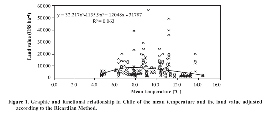
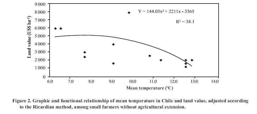
  ^a Includes irrigated and non-irrigated lands.

The typical curve generated by the RM for the T1 regression, which relates temperature to the land value of the totality of farmers can be observed in Figure 1.  The highest estimated land values tended to be concentrated in farms located in zones with moderate average temperatures of approximately 7-9 ºC. The agricultural systems with a lower land value were located in zones with more extreme average annual temperatures.  Figure 2 presents the best adjustment between the variables mean temperature versus land value (regression T9; R² = 38%), achieved with small-scale producers who do not receive agricultural extension services.  

Eleven regressions were calculated (P1 a P11) that relate the independent climatic variable precipitation to the estimated land value (Table 3). P1 explains 21% (R²) of the variation of the land value when the total of farms surveyed is analyzed. In general, there was more adjustment than in the analysis with the variable temperature. Nevertheless, in contrast to what was obtained with the temperature variable, among small-scale producers (P2) a lower R² was detected (11%) than among medium/large scale-producers (P3; R² = 30%). This could be related to a greater average productivity of the medium/large-scale producers, but with greater sensitivity to precipitation, given a greater spatial variability among their farms. As well, it could be related to the greater marginality of the small-scale producers, so the lower the expected yields, the less relative variation in response to changes in precipitation.

Table 3. Regressions (P1 to P11) generated by the Ricardian Method. Precipitation vs. land value (Y), considering small and medium/large producers, irrigated or non-irrigated land and with or without agricultural extension services.

Cuadro 3. Regresiones (P1 a P11) generadas por el Método Ricardiano. Precipitación vs. valor del suelo (Y), considerando productores pequeños y medianos/grandes, suelo irrigado o no irrigado, y extensión agrícola. 

^a Includes irrigated and non-irrigated lands.

Table 4. Relative change (%) of land value under different simulated scenarios of variation of temperature and precipitation.

Cuadro 4. Cambio relativo (%) del valor del suelo bajo diferentes escenarios simulados de variación de temperatura y precipitación. 

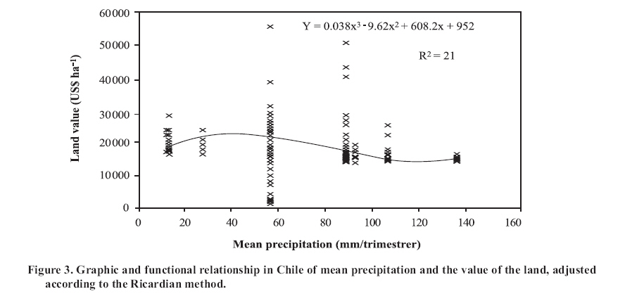
In the scenarios with agricultural extension (P8, P9, P10 and P11) a stronger relation or dependence was found with precipitation when there was not technical support to small-scale producers (P9; R² = 17%). On the other hand, with medium/large scale producers, the RM explained more the variation in the land value when there is technological training (P10). The causes of this result are not clear, but it could be that training of this strata (medium/large scale) is intense and with broad farm coverage in factors of management and inputs, but it is not the same with the massive implementation of irrigation, for example, in the southern zone of the country, which could generate sensitivity to variation in precipitation. Higher in R² was observed in the regressions of medium/large-scale producers, tending to be lower when there was not technical support (Table 3); so that this would suggest that with technical assistance small-scale producers could attenuate the effects of precipitation that in larger scale producers. This encourages strategies for the peasant producer related to the factor of precipitation and associated technologies.  

The typical RM curve generated with the totality of producers, where the highest estimated land values of land are concentrated in farms with moderate average precipitation, on the order of 60 mm per trimester, can be observed in Figure 3. The agricultural systems with lower land value, and probably less productivity and greater dependence on the factor of precipitation, are in zones with more extreme average levels of precipitation.                                                                                         

In general in Chile, the effects of simulated climatic change could affect some scenarios, strata of producers and zones of the country; the effects are seen as having less magnitude than is predicted in other parts of the continent. For example, Mendelsohn (1996) has estimated a negative impact on important agricultural sectors in Brazil, with strong economic implications, owing to the predominance of climates that are already very warm, which are more sensitive than temperate zones such as in Chile.  In this context, the average temperature in Chile is moderate to low in comparison to the rest of Latin America, with an annual average of 13.7 ºC; 14.4 ºC in summer and 4.6 ºC in winter. The annual average accumulated precipitation is 735 mm, with a range in the area studied of 21.8 mm (central north) to 1,350 mm (south) (Novoa et al., 1989).

The effects of the simulated scenarios are presented in Tables 4 and 5. Considering the totality of farmers, the scenarios that only increase temperature generate a moderately positive effect on the land value, with a maximum (1.48%) with a simulated increase of 5 ºC above the current national average temperature; this could reflect the fact that the area under study has a large surface (central south and south) with medium to low temperatures, whose production systems, mainly cattle raising, could be favored slightly. With changes in precipitation, effects of greater magnitude are obtained, and in some cases in the opposite sense of the variation in temperature; when precipitation is increased, land value increases slightly (6.9%), a symmetric situation is observed upon reducing precipitation. The influence of systems of greater productivity in the central and northern zones could be manifesting themselves, where precipitation levels are low and concentrated in winter, and which tends to offset the effect of the contrary reality that exists in the south of the country.

The scenarios that combine changes in temperature and precipitation support the described tendencies. When precipitation increases there is a moderate increase in land value (8%), independent of the increase in temperature.  On the other hand, the land devalues (6%) when precipitation decreases (Tables 4 and 5). The encountered behavior can be contradictory, with the perception that climatic change will always affect the agricultural sector negatively. Nevertheless, the possible moderate positive effects indicated were also detected by Alves and Evenson (1996) and Sanghi et al. (1997) in Brazil, in which the dependent variable of profitability showed a negative effect in central western region of the country, but also reflected beneficial effects in southern zones of Brazil, whose temperate climate is similar to Chile’s.  

The impact according to the producer stratum is also shown in Tables 4 and 5.  Among small-scale producers, land value follows a similar pattern to that of the total group of farmers surveyed. The greatest impact is in simulated scenarios that increase temperature and precipitation, with a 6% increase in land value. In other scenarios, the relative changes in land value are on the order of 3% when temperature increases and 2.5% when precipitation varies. Land value does not change when temperature increases and precipitation decreases. The predicted result in this stratum could respond to the presence of small-scale producers with marginal lands of lower productivity, consequently changes in temperature and precipitation can have a relatively minor impact. This could also reflect the existence in the central northern, central and central southern zones of small-scale producers who adopt a level of technology with a major intra-farm coverage, because of which they perceive less dependence of their management on climatic phenomenon.  As well, this could indicate that small farms have more stable land values because of scale, with fewer profitable alternatives in the use of the land.                               

Among the medium and large scale producers, land value also increases moderately in the scenarios that increase temperature, although it reaches an increase of 23% with the scenario in which temperature increases by 5 ºC.With scenarios that simulate changes in precipitation, the effects are more marked than among small-scale producers and the totality of survey respondents. An increase in precipitation would generate a reduction (28%) of the land value; while a contrary effect would be produced by reducing precipitation. Two realities of national agriculture could explain this behavior; on one hand in the northern, central northern and part of the central southern central zones, high technology production of export fruit predominates, which is highly susceptible to damage and increases in costs with excessive and unexpected rainfalls, which can generate a strong aversion to such phenomena among these producers. Parallel to this, in the southern zone cattle production predominates under conditions of high rainfall, so that a scenario of increased precipitation could have a negative perspective in terms of future profitability, causing greater complications and costs in the management of cattle, pastures, and soil adaptation and drainage.           

The scenarios that increase temperature and precipitation also show a reduction in the land value, although more attenuated (-5%), possibly because of the partially beneficial effect of the increase in temperature.  The scenarios that combine increased temperature and a reduction in precipitation generate a theoretic increase in the land value in a surprising range of 40 to 50%. This can respond to similar explanations to those presented for the scenarios in which only the level of precipitation changes.

In general, the behavior of the totality of farmers in the study show tendencies and magnitudes more similar to the stratum of small-scale producers than those of medium/large scale producers. This is probably because the majority of the surveyed producers belong to this stratum. The tendencies, compared in the columns of Tables 4 and 5, while in some scenarios seem contradictory, can or are reflecting dissimilar contexts among types or stratum of producers.

CONCLUSIONS

• There is in Chile a relationship between climatic variables and economic variables of the agricultural production systems.
• The Ricardian Method could explain satisfactorily (R² = 38%) the total national variation of the variable agricultural land value in response to climatic change. The independent variable temperature presented a lower relationship to land value than the independent variable precipitation. With additional restrictions, such as the presence or absence of irrigation or agricultural extension, diverse relationships were detected that require more specific analysis.                                    
• The scenarios of change in temperature and precipitation show less impact on the land value than has been reported for warmer regions of America. Predictions at the national level reflect neutral impacts with a slight tendency to be beneficial when temperature increases. With an increase in precipitation, the impact is of greater magnitude, from neutral to slightly favorable in small-scale agricultural producers and negative in medium and large-scale producers.
• Preliminary results were generated for discussion of the impact of climatic change on agriculture, with variations that could initially alert or orient effective strategies and policies of adaptation.  Decision-making should discriminate climatic, social-economic technical, size and productive situations.
• The Ricardian Method presented a promising level of adjustment to the Chilean situation, with the generation of regressions, climate-economic relations variables, response curves and simulation of scenarios.  The independent variables that gave a greater explanatory level of the dependent variable, the value of agricultural land, were spring temperatures, autumn temperatures and precipitation, the slope of the land and winter temperatures.   

ACKNOWLEDGEMENTS

This work was carried out as part of the project “Support to the Plan for the Study of the Impact of Global Warming in Latin American Countries as part of Climate and Rural Poverty: The Incorporation of Climate in Strategies of Rural Development” (SACPR), carried out jointly by Yale University (USA), IICA/PROCISUR, the World Bank, INIA Chile, INIA Uruguay, INTA Argentina, EMBRAPA Brazil, INIAP Ecuador, INIA Venezuela and CORPOICA Colombia.

The authors thank the Programmer and Statistical Technician, José Cares G., of INIA CRI Quilamapu, for his work and collaboration.

LITERATURE CITED

• Alves, D., and R.E. Evenson. 1996. Global warming impacts on Brazilian agriculture: estimates of the Ricardian Model. p. B30-B31. In Conference on environmetrics in Brazil, São Paulo. Instituto de Matemática e Estadística, Universidade de São Paulo, São Paulo, Brazil.
• Banco Central. 2006. Estudios económicos estadísticos. Banco Central de Chile. Disponible en http://www.bcentral cl/esp  Leído febrero 2007.
• CGIAR. 1998. CGIAR Mid-Term Meeting 1998: preliminary end-of-meeting report. Consultive Group for International Agricultural Research (CGIAR), Washington D.C., USA.  
• Dinar, A., R. Mendelsohn, R. Evenson, J. Parikh, A. Sanghi, K. Kumar, et al. (eds.) 1998. Measuring the impact of climate change on Indian agriculture. Technical Paper No. 402. World Bank, Washington D.C., USA. 
• European Commission. 1997. Climate change and agriculture in Europe: assessment of impacts and adaptations: Summary Report. 37 p. European Commission, Luxembourg, Grand Duchy of Luxembourg.
• Gujarati, D.N. 1996. Econometría. Capítulo 5. p. 102-139. 2ª ed. Regresión con dos variables: estimación por intervalos y prueba de hipótesis. McGraw-Hill Interamericana, D.F. México. 
• INE. 2006. Instituto Nacional de Estadísticas (INE), Santiago, Chile. Disponible en http://www.ine.cl Leído mayo 2007.
• Jones, J.W., N.B. Pickering, C. Rosenzweig, and K.J. Boote. 1997. Simulated impacts of global change on crops. p. 411-434. Technical Bulletin Nº 100. University of Florida, Gainsville, Florida, USA.
• Kumar, K., and J. Parikh. 2001. Indian agriculture and climate sensitivity. Global Environmental Change 11:147-154. The agriculture and the climatic change: the function of the FAO. Available in http://www.fao.org/Noticias/1997/971201.  Accessed 19 May 2006.
• Maddison, D. 2000. A hedonic analysis of agricultural land prices in England and Wales. Eur. Rev. Agric. Econ. 27:519-532.
• Mendelsohn, R. 1996. Estimating the market impacts of global warming in Brazil. 63 p. In Conference on environmetrics in Brazil, São Paulo. Abstracts. Instituto de Matemática e Estadística, Universidade de São Paulo, São Paulo, Brazil.
• Mendelsohn, R. 1999. Efficient adaptation to climate change. Climatic Change 45:583-600.
• Mendelsohn, R. (ed). 2001. Global warming and the American economy: A regional assessment of climate change. 224 p. Edward Elgar Publishing, Cheltenham, United Kingdom.
• Mendelsohn, R., A. Dinar, and A. Sanghi. 2001. The effect of development on the climate sensitivity of agriculture. Environment and Development Economics 6:85-101.
• Mendelsohn, R., Nordhaus.W. and D. Shaw. 1994. The impact of global warming in agriculture: A. Ricardian analysis. American Economic Review 84:772-780.
• Mendelsohn, R., W. Nordhaus, and D. Shaw. 1994. Measuring the impact of global warming on agriculture. Am. Econ. Rev. 84:753-771.
• Novoa, R., V. Sergio, and P. Del Canto. 1989. Mapa agroclimático de Chile. 221 p. Instituto de Investigaciones Agropecuarias, Santiago, Chile.
• ODEPA. 2000. La agricultura chilena del 2010. Tres visiones sociopolíticas. 238 p. Oficina de Estudios y Políticas Agrarias (ODEPA), Santiago, Chile.
• ODEPA. 2006. Oficina de Estudios y Políticas Agrarias (ODEPA). Disponible en http://www.odepa.gob.cl. Leído noviembre 2006.
• Reinsborough, A. 2003. A Ricardian model of climate change in Canada. Can. J. Econ. 36:21-40.
• Rosenzweig, C., and A. Iglesias (eds.) 1994. Implications of climate change for international agriculture: crop modeling study. p. 94-103. July. Environmental Protection Agency (EPA), Washington D.C.,  U.S.A.
• Rosenzweig, C., and M. Parry. 1994. Potential impact of climate change on world food supply. Nature 367:133-138.
• Sanghi, A., D. Alves, R. Evenson, and R. Mendelsohn. 1997. Global warming impacts on Brazilian agriculture: estimates of the Ricardian model. Universidad de São Paulo and Fundación de Pesquisas Económicas (FIPE), São Paulo, Brazil. Economía Aplicada 1(1):7-34.
• SAS. 1999. SAS//STAT. Guide for personal computers. Version 8.0. 1028 p. SAS Institute Inc., Cary, North Carolina, USA.
• Siqueira, O., J.R. Farias, and L.M. Sans. 1994. Potential effects of global climate change for Brazilian agriculture: applied simulation studies for wheat, maize and soybeans. Revista Brazileira de Agrometeorología 2:115-129.

Copyright 2008 - Instituto de Investigaciones Agropecuarias, INIA (Chile).

The following images related to this document are available:

Photo images