Chilean Journal of Agricultural Research Instituto de Investigaciones Agropecuarias, INIA ISSN: 0718-5820 EISSN: 0718-5839 Vol. 68, Num. 1, 2008, pp. 69-79

Chilean Journal of Agricultural Research (formerly Agricultura Técnica), Vol. 68, No. 1, Jan-March, 2007 pp. 69-79

Research

A Ricardian Analysis Of The Impact Of Climate Change On South American Farms

Análisis Ricardiano del impacto del cambio climático en predios agrícolas en Sudamérica

S. Niggol Seo[1]^* and Robert Mendelsohn¹

[1]Yale University, School of Forestry and Environmental Studies, 230 Prospect St., New Haven, Connecticut, 06511, USA. E-mail: niggol.seo@aya.yale.edu; robert.mendelsohn@yale.edu  *Corresponding author.

Received: 5 May 2007.
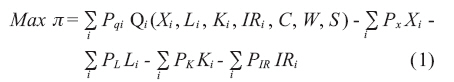
Accepted: 2 August 2007.

Code Number: cj08007

ABSTRACT

 This study estimates the impact of climate change on South American agriculture taking into account farm adaptations. The study used a Ricardian analysis of 2300 farms to explore the effects of global warming on land values. In order to predict climate change impacts for this century, were examined climate change scenarios predicted by three Atmospheric Oceanic General Circulation Models (AOGCM): the Canadian Climate Center (CCC), the Centre for Climate System Research (CCSR), and the Parallel Climate Model (PCM) models. Several econometric specifications were tested, and five separate regressions were run: for all farms, small household farms, large commercial farms, rainfed farms, and irrigated farms. Farmland values will decrease as temperature increases, but also as rainfall increases except for the case of irrigated farms. Under the severe Canadian Climate Center (CCC) scenario, South American farmers will lose on average 14% of their income by the year 2020, 20% by 2060, and 53% by 2100, but half of these estimates under the less severe Centre for Climate System Research (CCSR) scenario. However, farms will lose only small amounts of income under the mild and wet Parallel Climate Model (PCM) scenario. Both small household farms and large commercial farms are highly vulnerable, but small farms are more vulnerable to warming, while large farms are more vulnerable to rainfall increases.  Both rainfed and irrigated farms will lose their incomes by more than 50% by 2100, with slightly more severe damage to irrigated farms, but the subsample analysis treats irrigation as exogenous.

Key words: climate change, agriculture, Ricardian approach, South America.

RESUMEN

En este estudio se estimó el impacto del cambio climático sobre la agricultura de Sudamérica considerando la adaptación de los predios. Usando el Método Ricardiano se realizó un análisis de 2300 predios para explorar los efectos sobre el valor de la tierra. Con el objeto de predecir los impactos del cambio climático en el presente siglo, se examinaron tres escenarios que predice el Modelo de Circulación General Atmosférico Oceánico (AOGCM): el escenario del Centro Canadiense del Clima (CCC), el del Centro para Investigación de Sistemas Climáticos (CCSR), y el del Modelo de Clima Paralelo (PCM). Se evaluaron varias especificaciones econométricas, y se realizaron cinco regresiones: todos los predios, predios pequeños, predios comerciales, predios de secano y predios con riego. El valor de la tierra agrícola disminuirá a medida que incrementa la temperatura y la lluvia, excepto en el caso de los predios regados. Bajo el severo escenario del CCC, los agricultores sudamericanos perderán 14% de sus ingresos el año 2020, 20% el año 2060, y 53 % el año 2100, y solo la mitad bajo el menos severo escenario de CCSR. Sin embargo, los predios perderán pequeños márgenes bajo el escenario suave y húmedo del PCM. Tanto los predios pequeños como los grandes son altamente vulnerables, pero los pequeños son más vulnerables mientras que los grandes son mas sensibles a un aumento de la precipitación. Los predios de secano y los de riego perderán más del 50% de sus ingresos el año 2100, con mayores daños los predios regados, pero la submuestra trata el riego como un factor exógeno.

Palabras clave: cambio climático, agricultura, Método Ricardiano, Sudamérica.

INTRODUCTION

 A growing number of studies indicate that the world is warming and will continue to warm as the concentration of greenhouse gases rises in the future (IPCC, 2001a; 2007). However, there remains considerable debate about how harmful climate change will actually be (IPCC, 2001b). This paper examines the impact of climate change on agriculture in South America. Agriculture accounts for 8.6% of Gross Domestic Product (GDP) in South America (World Bank, 2004) and uses approximately one third of the land area of the continent (World Resources, 2005). Farmers are already highly vulnerable because of high current temperatures and poverty in rural areas. There have been several country level agronomic studies of selected crops in South America that suggested key crops would be severely damaged by higher temperatures (IPCC 2001b), but there have been very few agroeconomic studies. An economic study in Brazil indicated that farm land values would fall with warming, but the magnitude of the effects was much smaller than the previous estimates from agronomic studies (Mendelsohn et al., 2001). In addition, agronomists have expressed concern that small household farms may be especially vulnerable because of poverty and lack of alternatives (Rosenzweig and Hillel, 2005).    

 This study is the first continental scale study of climate change impacts on agriculture in South America. The analysis measures the sensitivity of land value per hectare to seasonal temperatures and precipitations. The empirical research relies on surveys of 2300 farmers in seven countries across South America. The surveys were collected in collaboration with teams from each country. Additional data on soils, climates, and future climate scenarios were collected from various other sources. The Ricardian approach was then applied to measure the sensitivity of land value per hectare to climate and other factors (Mendelsohn et al., 1994). Several functional forms were estimated to test the robustness of the results. In addition, this study provides one of the first formal tests of whether small household farms are more sensitive to climate than large commercial farms. The study also tests whether rainfed and irrigated farms have similar climate sensitivities. The estimated parameters from the Ricardian regressions were then used to simulate climate change impacts based on a set of climate change scenarios for the future. The projections are intended to provide a sense of what climate change alone will do in the future.

METHODOLOGY

The Ricardian model assumes that each farmer wishes to maximize income subject to the exogenous conditions of their farm. Specifically, the farmer chooses the crop or livestock and inputs for each unit of land that maximizes income, as is expressed in Equation 1 (Mendelsohn et al., 1994):

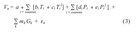
where π is net annual income, P_qi is the market price of crop (or livestock) i, Q_i is a production function for crop i, X_i is a vector of annual inputs, such as seeds, fertilizer, and pesticides for each crop i, L_i is a vector of labor (hired and household) for each crop i, K_i is a vector of capital, such as tractors and harvesting equipment for each crop i , C is a vector of climate variables, IR_i is a vector of irrigation choices for each crop i, W is available water for irrigation, S is a vector of soil characteristics, P_x is a vector of prices for the annual inputs, P_L is a vector of prices for each type of labor, P_K is the rental price of capital, and P_IR is the annual cost of each type of irrigation system.

If the farmer chooses the crop or livestock that provides the highest net income and chooses each endogenous input in order to maximize net income, the resulting chosen net income will be a function of just the exogenous variables (Equation 2; Mendelsohn et al., 1994):  

π* = f (P_q , C, W, S, P_x , P_L , P_K , P_IR )                                            (2)

With perfect competition for land, free entry and exit will ensure that excess profits are driven to zero. Land rents will consequently be equal to net income per hectare (D. Ricardo, 1817; Mendelsohn et al., 1994). Land value will then reflect the present value of net income for each farm. Of course, if a farm which is located near a city is expected to be converted to another land use, for example, to be developed into an urban city, this will also affect its land value. Consequently, Ricardian analyses must be careful measuring farmland values near cities.                          

The Ricardian model was developed to explain the variation in land value per hectare of cropland over climate zones (Mendelsohn et al., 1994). In several studies, the land value per hectare of cropland has been found to be sensitive to seasonal precipitation and temperature (Mendelsohn et al., 1994, 1999, 2001; Dinar et al., 1998; Mendelsohn 2001; Mendelsohn and Dinar, 2003; Seo et al., 2005; 2008). Similar results have also been found for crop net revenue (Kurukulasuirya et al., 2006) and livestock net revenue (Seo and Mendelsohn, 2008a, 2008b). Because the response is nonlinear, a quadratic functional form has been used in every Ricardian study. Consequently, we estimated the following equation:

where the dependent variable is land value per hectare of land, T and P represent temperature and precipitation variables, G represents a set of relevant socio-economic variables, ε is an error term, and the other parameters are coefficients.  In this paper, we rely on seasonal temperature and precipitation variables, not heating degree days during the growing season, because the growing season changes with location and because we did not have an accurate measure of heating degree days available in South America

 In order to test the robustness of the model, we explored several different econometric specifications of equation 3. We compared a four-season specification to a two-season specification. We added climate interaction terms between temperature and precipitation. The climate effects on small household farms and large commercial farms were separated. This tests the assumption that small household farms are more vulnerable than large commercial farms to climate change because they have fewer substitution alternatives. We also included country dummies to see whether there are hidden variables concerning each country that affect the results. In addition, we estimated separate regressions for rainfed and irrigated farms using the best specification from the above five (Schlenker et al., 2005). These regressions assumed that irrigation is exogenous. In subsequent papers, we explored the implications of irrigation being endogenous (Mendelsohn and Seo, 2007).  

The impact of climate change is measured by the change in land value. The change in land value, ΔV, resulting from a climate change from C₀ to C₁ can be measured as follows:

The Ricardian function in equation 3 is intended to be a locus of the most profitable crops with respect to each exogenous variable, such as temperature. It is estimated across crops and across inputs, revealing the net effect of changing the exogenous variable. Because farmers are assumed to make adaptations that are profitable, the method automatically captures the adaptation inherent in the market (Mendelsohn et al., 1994). This is an important distinction and sets this approach distinctly apart from studies that do not take adaptation into account (Deschenes and Greenstone, 2007).

 There have been a number of criticisms of the Ricardian approach over the years since it was first developed. There was initially a concern about irrigation (Cline 1996; Schenkler et al., 2005). However, this study and other analyses (Kurukulasuriya and Mendelsohn, 2006; Mendelsohn and Seo, 2007) now address this question carefully. There have also been concerns about the role of price changes (Quiggin and Horowitz, 1999). Although changes in local supply might be dramatic, prices of food crops tend to be determined by global markets. With the expansion of crop production in some parts of the world and the contraction in others, the changes in the price of crops from global warming is expected to be small (Reilly et al., 1994). Finally, there is a concern that the Ricardian analysis does not take into account the cost of transition (Kelly et al., 2005). Although we expect transition costs to be relatively small, the Ricardian method does not measure them.        

DATA

Economic data was collected by country teams from seven countries: Argentina, Uruguay, Chile, and Brazil from the Southern Cone region, and Venezuela, Ecuador, and Colombia from the Andean region. The countries were selected to cover a wide range of climate zones and given the availability of researchers. Districts were explicitly selected to capture a wide range of climates within each country. However, climates that could not support any agriculture were not surveyed. In each country, 15-30 districts were selected and 20-30 households were randomly chosen in each district. Cluster sampling in the districts was done to control the cost of the survey. The surveys asked questions about farming activities, both crop production and livestock production, during the period from July 2003 to June 2004.  

The climate data come from two sources: satellite temperature observations from the U.S. Defense Department (Basist et al., 1998) and rainfall observations from the World Meteorological Organization (WMO, 1989). In earlier comparisons across Brazil, it was found that the temperature measurements from the satellite were superior to the interpolated weather station measurements (Mendelsohn et al., 2007a). Most rural areas do not have a weather station nearby and so require interpolation. The satellites make direct observations over the entire land area using microwave imagers. These measurements are very effective for capturing temperature, but cannot directly capture precipitation. Satellites can measure soil wetness, but this index is inferior to the interpolated station measurements of precipitation because the former is influenced by irrigation, large water bodies, and dense forests (Mendelsohn et al.,2007a).

Soil data were obtained from the Food and Agriculture Organization digital soil map of the world (FAO, 2003). The data were extrapolated to the district level using a Geographical Information System. The data set reports 26 major soil groups, soil texture, and land slope at the district level.

In order to predict climate change impacts for the coming century, we examined climate change scenarios predicted by three Atmospheric Oceanic General Circulation Models (AOGCM’s). We rely on these three scenarios to reflect the wide range of plausible outcomes predicted by the Intergovernmental Panel on Climate Change (IPCC, 2007). Specifically, we use the A1 scenarios from the following models: Canadian Climate Center (CCC) (Boer et al., 2000), Center for Climate System Research (CCSR) (Emori et al., 1999), and Parallel Climate Model (PCM) (Washington et al., 2000). For each scenario, a country-specific forecast is generated by weighting each model grid zone by its population.

RESULTS

The analysis was inclusive of all the crops in the region. The most important crops were cereals (wheat, maize [Zea mays L.], barley [Hordeum vulgare L.], rice [Oryza sativa L.], oats [Avena sativa L.]), oil seeds (soybean [Glycine max (L.) Merr.], peanuts [Arachis hypogaea L.], sunflower [Helianthus annuus L.]), vegetables/tubercles (potatoes [Solanum tuberosum L.], cassava [Manihot esculenta Crant]), a variety of perennial grasses, and specialty crops, such as cotton (Gossypium hirsutum L.), tobacco (Nicotiana rustica L.), tea (Camellia sinensis (L.) Kuntze), coffee (Coffea arabica L.), cacao (Theobroma bicolor Bonpl.), sugarcane (Saccharum sp.), and sugar beet (Beta vulgaris L.). Major tree/shrub crops include a large variety of fruits, oil palm (Elaeis guineensis Jacq.), and others. The analysis also included the value of livestock. South American farms rely a great deal on beef and dairy cattle but also have chickens, pigs, and sheep.

Although commercial agriculture and agro-industry businesses are well developed, there are many places in the continent that still rely on small household farming systems. In rural communities in the Andean valleys and plateaus, for example, small farms are part of subsistence lifestyles with heavy reliance on labor inputs. These small farms may be more sensitive to climate change than large commercial farms (Rosenzweig and Hillel, 1998). We test this hypothesis by examining the climate sensitivity of both small and large farms. Small farms were defined as farms that produce mainly for their own use. 

 The regression of land values on climate and other control variables, with a chosen econometric specification for all types of farms in South America, is shown in the second column of Table 1. Several different econometric specifications were examined before we settled on the specification in Table 1 with two seasons and country fixed effects. The third and fourth columns of the table show separate regressions of small household farms and large commercial farms. The fifth and sixth columns of the table show separate regressions of rainfed farms and irrigated farms. For the specifications tested, we used the same soil and socio-economic variables and the same quadratic relationship between climate variables and land value. The first specification was a two-season model with summer and winter temperatures and precipitation. The second specification had four seasons, adding spring and fall. The third specification added climate interaction terms. The final specification added country dummies to test country fixed effects.  The comparison of the two-season specification to the four-season specification revealed that only a few climate coefficients in the four-season model were significant. The two-season specification appeared to capture the important seasonal effects of climate. In the next specification, we tested whether climate interactions between temperature and precipitation are important. In general, summer and winter climate interaction terms were not significant and made the regressions unstable. In the final specification, we added country dummies, excluding Brazil, to test country fixed effects, which are common due to differing development stages of each country and different public policies. The results indicated that country fixed effects are significant.

Table 1. Ricardian regressions for all farms and subsamples by commercialization and by irrigation. 2004-2005.

Cuadro 1. Regresión Ricardiana para todos los predios y submuestras por comercialización y riego. 2004-2005.

*: denotes significance at 5% level; Temp.=Temperature; Prec.=Precipitation.
The dependent variable is land value in USD per hectare of land in 2003-2004.

 Most climate variables in the whole sample analysis shown in the second column of Table 1 were significant. The separate regressions of small household farms and large commercial farms also indicated that land values of these farms were highly sensitive to climate. Small farms were sensitive to winter temperature and summer and winter precipitations, whereas large farms were sensitive only to summer and winter precipitations. Across the three regressions in Table 1 (2^nd, 3^rd, and 4^th columns), country dummies were significant and negative in contrast to Brazil, except for positive but insignificant estimates for Colombia and Venezuela. Among the control variables, farms with electricity have higher land values. Soils such as Ferralsols and Phaeozems are associated with higher land values, while Cambisols with lower land values. When the soil texture is clay, farmland values are lower. When the terrain is flat, the farm commands higher land values in contrast to farms in steep locations.

 Since the quadratic functional form made it difficult to interpret the effects of changes in the climate coefficients, we calculated annual marginal effects of climate change in Table 2 for the first three regressions in Table 1. For the regression of the whole sample, a temperature increase by 1 °C decreased farmland values on average by 175 USD per hectare. Small household farms were slightly more vulnerable to higher temperature than large commercial farms according to separate regressions on the corresponding subsamples, which confirms the original hypothesis that small farms could be affected by global warming more heavily. A precipitation increase was also harmful across the three different regressions. Large commercial farms were more vulnerable to higher precipitation by 1 mm/month than small household farms. Large commercial farms, such as beef cattle farms in Argentina often owned commercial livestock, which do not perform well when precipitation increases (Seo and Mendelsohn, 2008a, 2008b). All the marginal effects and elasticity estimates in Table 2 were significant at 5% level, except for the rainfall effect from the small household farm regression.

Table 2. Marginal effects and elasticities (USD ha^-1) for the whole sample and subsamples by size and irrigation. 2003-2004.

Cuasdro 2. Efectos marginales y elasticidades (USD ha^-1) para la muestra completa y submuestras según tamaño y uso de riego. 2003-2004.

Marginal effects are changes in land value (USD) from temperature increase of 1 °C or rainfall increase by 1 mm at the mean of the samples. Elasticities are corresponding percentage changes in land values.
Calculated from the coefficients in Table 1 at the mean of the corresponding samples.
*: denotes significance at 5% level.

Separate analyses on rainfed farms and irrigated farms were conducted (fifth and sixth columns in Table 1). Separate regressions were run for 1570 rainfed farms and 465 irrigated farms using the same econometric specification as above. The regression parameter estimates of the rainfed farm model in the fifth column are similar to those of the all farm model in the second column of the table. However, rainfed farm land values were not sensitive to temperatures, but only to precipitation. The regression from the irrigated farm model resulted in slightly different estimates. Most notably, the estimate of clay soils is positive and significant, and the estimate of the Venezuela dummy is negative, but not significant. This implies that an irrigation system is more effective in clay soils than in sandy soils. Irrigated farms are more sensitive to both summer and winter precipitations.

 The differences between the results from the rainfed farm model and those from the irrigated farm model can also be seen from the estimates of marginal effects and elasticities in Table 2. Irrigated farms were twice more vulnerable to temperature increase by 1 °C than rainfed farms were. A marginal increase in precipitation decreased rainfed farm land values significantly, but increased irrigated farm land values. However, the estimate is not significant. These estimates treat irrigation as exogenous.  

CLIMATE PROJECTIONS

 Using the climate parameter estimates from the previous section, we predicted climate change impacts over the coming century based on the following three Atmospheric Oceanic General Circulation Models (AOGCM’s): CCC, CCSR, and PCM. These three climate scenarios were chosen to represent the broad range of possible outcomes (IPCC, 2007). In each case, a country-specific forecast was generated by weighting the outcome in each model grid zone by its population. The South American mean temperature and rainfall predicted for the baseline year and in 2020, 2060, and 2100 were used to predict future land values. The models provided a range of predictions: PCM predicted a 1.9 °C increase, CCSR a 3.3 °C increase and CCC a 5.0 °C increase in annual mean temperature by 2100. The temperature projections of all the models steadily increased over time from about a 1 ºC increase in 2020 to a 2.5 ºC increase in 2060 on average. The models also provided a range of rainfall predictions. PCM predicted a general increase of 10% in rainfall, whereas CCSR and CCC predicted a reduction of 5% and 10%, respectively by 2100. The rainfall predictions of the models did not steadily increase, but rather had a noisy pattern over time. For example, PCM predicted an initial rainfall increase by 2020, but a decrease by 2060, and an increase again by 2100. The actual climate change predictions used in the analysis were country-specific. For example, even though the mean rainfall for South America might increase/decrease, some countries will nonetheless experience a reduction/increase in rainfall.

 For each climate scenario and each time period, the climate model’s predicted change to the baseline temperature in each district was added. The climate model’s predicted percentage increase in precipitation was multiplied to the baseline precipitation in each district or province. This gave a new climate for every district in South America. The land value per hectare of the baseline climate and each new climate were then computed. Subtracting the future land value estmates from the baseline land value estimates yielded a change in land value per hectare in each location.

 The second column of Table 3 shows the results from the whole sample regression in South America using the parameter estimates in the second column of Table 1.  With the Ricardian model of the entire sample, the CCC and CCSR scenarios in 2020 lead to a loss of land value of around 14%, but the PCM scenario leads to little change in the land value. This result from the PCM scenario was due to the rainfall increase under this scenario combined with a milder temperature increase. Under the three scenarios, estimated damages rise over time. According to the CCC scenario, farms will lose on average 20% of their land value by 2060, and 53% by 2100. The other two scenarios predicted similar changes, but with smaller magnitudes. These different predictions were largely due to the difference in predicted temperature change across the three models and the trends in precipitation change. The estimates from the CCC and CCSR scenarios were significant, but not significant in the case of the PCM scenario. 

Table 3. Climate change impacts from Atmospheric Oceanic General Circulation Model (AOGCM) climate scenarios (USD ha^-1): the Canadian Climate Center (CCC), the Centre for Climate System Research (CCSR) and the Parallel Climate Models (PCM).

Cuadro 3. Impactos del cambio climático según los escenarios de clima del Modelo de Circulación General Atmosférico Oceánico (AOGCM) (USD ha^-1): Canadian Climate Center (CCC), Centre for Climate System Research (CCSR) y Parallel Climate Model (PCM).

The estimates are changes in land value in USD per hectare of land calculated at the mean of the corresponding sample. *: denotes significance at 5% level.

Small household farms, shown in the third column of the Table 3, were estimated to lose a similarly large amount of income over time, but the losses were slightly smaller than those from the whole sample model in the second column in the table. On the other hand, large farms were predicted to lose similarly large amounts of income over time, losing more than small household farms. Large farms in general depend highly on livestock, which does not perform well under a wet condition, such as in PCM (Seo and Mendelsohn, 2008a; 2008b). 

 The estimates from the rainfed farm subsample and the irrigated farm subsample are shown in the fifth and sixth columns of Table 3, which indicate similarly large losses to both types of farms. The results from the rainfed farms were very close to those from the whole sample regression in the second column of the table. The results from the irrigated farm sample were quite different. Firstly, it predicts much larger losses to irrigated farms, 20% more loss in 2100. Even more distinct is that irrigated farms will lose their incomes from the PCM scenario as much as they will from the CCC scenario. It is dryland farms that benefit from more rainfall under this scenario. But the estimates from these subsamples treat irrigation as an exogenous choice.  

MAIN FINDINGS  

 This paper examined the vulnerability of South American agricultural production to climate change. Surveys of farms were collected across seven countries in South America. Farmland values were run against a set of climate variables, soils, and other socio-economic variables. Several different specifications were tested to demonstrate the robustness of the analysis. Using the final specification with two seasons and country fixed effects, we ran separate regressions for all farms, small household farms, and large commercial farms, to test whether small household farms are more vulnerable to climate change. Additional regressions were run separately for rainfed farms and irrigated farms. Across all the models, climate variables were significant determinants of farmland values in South America. Country dummies were significant. Farms with electricity had higher land values. When the soil texture was clay, farmland values were lower except in the irrigated farms. Farmland values were higher in flat terrains.

For the regression of all farms, a marginal temperature increase decreased farmland values so did a marginal increase in rainfall. Small household farms were slightly more vulnerable to higher temperature than large commercial farms, while large commercial farms were more vulnerable to higher precipitation. Hence, the original hypothesis that small farms were more vulnerable to climate change holds for temperature increase, but not for rainfall increase. Irrigated farms were twice more vulnerable to temperature increase by one degree Celsius than rainfed farms. A marginal increase in precipitation decreased rainfed farm land values significantly, but had little impact on irrigated farms.

The three climate predictions from the AOGCM scenarios were used to forecast changes in land values in the coming century. With the Ricardian model of the entire sample, the CCC and CCSR scenarios in 2020 led to a loss of land value of around 14%, but the PCM scenario led to little change in the land value. Under the three scenarios, estimated damages rose over time. According to the CCC scenario, farms will lose on average 20% of their land value by 2060, and 53% by 2100. Small household farms were estimated to lose similarly large amounts of income over time, but the losses were slightly smaller than those from the all farm model. On the other hand, large commercial farms were expected lose more than small household farms due to shifts in rainfall. The results from the rainfed farms were very close to those from the whole sample model. The results from the irrigated farm model, however, were quite different. Firstly, it predicted much larger losses to irrigated farms. In addition, irrigated farms were expected to lose their incomes from the PCM scenario as much as from the CCC scenario.

The loss of substantial net revenue from climate change is likely to reduce rural incomes substantially over the coming century (Mendelsohn et al., 2007b). Since urban sources of income may be relatively robust, there will likely be a growing gap between urban and rural incomes as a result of global warming. Countries and international agencies may want to direct resources at providing relief and new opportunities for the rural poor. They may also want to facilitate the continued migration of people from the countryside to more urban settings as part of a general development strategy.

There are a number of caveats that readers should keep in mind when interpreting these results. First, the cross sectional analysis is vulnerable to omitted variables. If important variables have been left out of the analysis and they are correlated with climate, they can bias the results. For example, the results do change slightly when country dummy variables are included. Second, the analysis did not consider carbon fertilization which is predicted to increase future crop productivity (Reilly et al., 1996). Third, the analysis did not include changes in prices. If some of the more severe scenarios come to pass, there may be changes in wages and other input and output prices. These price changes will reduce the severity of the damage to welfare. Fourth, the analysis did not take into account future technological change (Evenson and Gollin, 2003). In general, technological change is expected to increase overall crop and livestock productivity. However, technological change could be directed specifically to deal with higher temperatures or dryer conditions. For example, Brazil has developed a new soybean variety specifically to grow in the hot and dry conditions of the Mato Grosso region.

CONCLUSIONS

 This paper reveals that South American agriculture is highly vulnerable to climate change. If global warming is mild, the impact will be small. However, if severe warming scenarios come to pass, farmers could lose up to 50% of their net revenue by the end of this century. This would be a stunning blow to the agricultural sector in South America. The impact would be even more devastating to the hottest most vulnerable regions in South America. Both small household farms and large commercial farmers appear to be highly vulnerable to global warming scenarios with slightly larger damages to large commercial farms due to shifts in rainfall. Similarly, irrigated farms and rainfed farms are highly vulnerable with slightly more severe damage to irrigated farms.

There are a number of caveats that readers should keep in mind when interpreting these results. First, the cross sectional analysis is vulnerable to omitted variables; second, the analysis did not consider carbon fertilization which is predicted to increase future crop productivity; third, the analysis did not include changes in prices; and fourth, the analysis did not take into account future technological change.

ACKNOWLEDGEMENT

Funding of this project was provided by the World Bank. We thank Emilio Ruz, Flavio Avila, Jorge Lozanoff, Luis José María Irias, Jorge González, Flavio Játiva, Irma Baquero, Alfredo Albin, Bruno Llanfranco, and Rafael Pacheco for their contribution to this project. We would also like to thank Ariel Dinar for his support and leadership throughout this project. 

LITERATURE CITED

• Basist, A., N. Peterson, T. Peterson, and C. Williams. 1998. Using the special sensor microwave imager to monitor land surface temperature, wetness, and snow cover. J. Appl. Meteorol. 37:888-911.
• Boer, G., G. Flato, and D. Ramsden. 2000. A transient climate change simulation with greenhouse gas and aerosol forcing: projected climate for the 21^st century. Clim. Dynam. 16:427-450.
• Cline, W. 1996. The impact of global warming on agriculture: Comment. Am. Econ. Rev. 86:1309–1311.
• Deschenes, O., and M. Greenstone. 2007. The economic impacts of climate change: evidence from agricultural output and random fluctuations in weather. Am. Econ. Rev. 97:354-385.
• Dinar, A., R. Mendelsohn, R. Evenson, J. Parikh, A. Sanghi, and K. Kumar. (eds.) 1998. Measuring the impact of climate change on Indian agriculture. 266 p. World Bank Technical Paper No. 402. World Bank, Washington, D.C., USA.
• Emori, S., T. Nozawa, A. Abe-Ouchi, A. Namaguti, and M. Kimoto. 1999. Coupled ocean-atmospheric model experiments of future climate change with an explicit representation of sulfate aerosol scattering. J. Meteorol. Soc. Jpn. 77:1299-1307.
• Evenson, R., and D. Gollin. 2003. Assessing the impact of the Green Revolution, 1960-2000. Science 300:758-762.
• FAO. 2003. The digital soil map of the world (DSMW) CD-ROM. Food and Agriculture Organization, Italy, Rome. Available at http://www.fao.org/AG/agl/agll/dsmw.stm Accessed March 2004.
• IPCC. 2001a. The scientific basis. p. 881. In J. Houghton, Y. Ding, D. Griggs, M. Noguer, P. Van der Linden, X. Dai et al.(eds.) Climate change 2001. Contribution of Working Group II to the Third Assessment Report of the Intergovernmental Panel on Climate Change. Cambridge University Press, Cambridge, UK.
• IPCC.  2001b. Impacts, adaptation, and vulnerability. p. 1032. In McCarthy, J., O. Canziani, N. Leary, D. Dokken, and K. White (eds.) Climate change 2001. Contribution of Working Group II to the Third Assessment Report of the Intergovernmental Panel on Climate Change (IPCC).Cambridge University Press, Cambridge, UK.
• IPCC. 2007. Summary for Policymakers. In Solomon, S., D. Qin, M. Manning, Z. Chen, M. Marquis, K.B. Averyt, M. Tignor and H.L. Miller (eds.) Climate change 2007: The physical science basis. Contribution of Working Group I to the Fourth Assessment Report of the Intergovernmental Panel on Climate Change. Cambridge University Press, Cambridge, UK.
• Kelly, D.L., C. Kolstad, and G.T. Mitchell. 2005. Adjustment costs from climate change. J. Environ. Econ. Manag.50:468-95.
• Kurukulasuriya, P., R. Mendelsohn, R. Hassan, J. Benhin, M. Diop, H. M. Eid, K.Y. Fosu, G. Gbetibouo, S. Jain, , A. Mahamadou, S. El-Marsafawy, S. Ouda, M. Ouedraogo, I. Sène, D. Maddision, S. N. Seo and A. Dinar.2006. Will African agriculture survive climate change? World Bank Econ. Rev. 20(3):367-388.
• Kurukulasuriya, P., and R. Mendelsohn. 2006. Modeling endogenous irrigation: The impact of climate change on farmers in Africa. Center for Environmental Economics and Policy in Africa (CEEPA) Discussion Paper No. 8. Special Series on Climate Change and Agriculture in Africa.
• Mendelsohn, R., W. Nordhaus, and D. Shaw. 1994. The impact of global warming on agriculture: A Ricardian analysis. Am. Econ. Rev. 84:753-771.
• Mendelsohn, R., W. Nordhaus, and D. Shaw. 1999. The impact of climate variation on U.S. agriculture. p. 55-74. InMendelsohn, R., and J. Neumann. (eds). The economic impact of climate change on the economy of the United States. Cambridge University Press, Cambridge, UK.
• Mendelsohn, R. (ed) 2001. Global Warming and the American Economy: A Regional Analysis. Edward Elgar Publishing, UK.
• Mendelsohn, R., A. Dinar, and A. Sanghi. 2001. The effect of development on the climate sensitivity of agriculture. Environ. Dev. Econ. 6:85-101.
• Mendelsohn, R., and A. Dinar. 2003. Climate, water, and agriculture. Land Econ. 79:328-341.
• Mendelsohn, R., A. Basist, F. Kogan, and P. Kurukulasuriya. 2007a. Climate analysis with satellite versus weather station data. Clim. Change 81:71-83.
• Mendelsohn, R., A. Basist, P. Kurukulasuriya, and A. Dinar. 2007b. Climate and rural income. Clim. Change 81:101-118.
• Mendelsohn R., and S.N. Seo. 2007. An integrated farm model of crops and livestock: Modeling Latin American agricultural impacts and adaptations to climate change. World Bank Policy Research Series Working Paper 4161. 41 p. World Bank, Washington DC., USA.
• Quiggin, J. and J. Horowitz. 1999. The impact of global warming on agriculture: A Ricardian analysis: A Comment. Am. Econ. Rev. 89(4): 1044-1045.
• Reilly, J., W. Baethgen, F. Chege, , S. van de Geijn, L. Enda, A. Iglesias, G. Kenny, D. Patterson, J. Rogasik, R. Rotter, C. Rosenzweig, W. Sombroek, and J. Westbrook. 1996. Agriculture in a changing climate: impacts and adaptations. p. 427-468. In Watson, R., M. Zinyowera, R. Moss, and D. Dokken (eds) Climate Change 1995: Intergovernmental Panel on Climate Change Impacts, Adaptations, and Mitigation of Climate Change. Cambridge University Press, Cambridge, UK  
• Reilly, J., N. Hohmann, and S. Kane. 1994. Climate change and agricultural trade: who benefits, who loses? Global Environ. Chang. 4(1):24-36.
• Ricardo, D. 1817. On the principles of political economy and taxation. John Murray, London, England.
• Rosenzweig, C., and D. Hillel. 1998. Climate change and the global harvest: potential impacts of the greenhouse effect on agriculture. Oxford University Press, New York, USA.
• Rosenzweig, C., and D. Hillel. 2005: Climate change, agriculture and sustainability. p. 243-268. In Lal, R., N. Uphoff, B.A. Stewart, and D.O. Hansen (eds.) Climate change and global food security. Taylor & Francis, London, UK.
• Schenkler, W., M. Hanemann, M., and A. Fisher. 2005. Will U.S. agriculture really benefit from global warming? Accounting for irrigation in the hedonic approach. Am. Econ. Rev. 95:395-406
• Seo, S. N., R. Mendelsohn, and M. Munasinghe. 2005. Climate change and agriculture in Sri Lanka: A Ricardian valuation. Environ. Dev. Econ.10:581-596.
• Seo, S.N., and R. Mendelsohn. 2008a. Climate change impacts and adaptations on animal husbandry in Africa. African Journal of Agricultural and Resource Economics (in press).
• Seo, S.N., and R. Mendelsohn. 2008b. Measuring impacts and adaptations to climate change: A structural Ricardian model of livestock management in Africa. Agr. Econ. 38:1-15.
• Seo, N.S., R. Mendelsohn, A. Dinar, R. Hassan, and P. Kurukulasuriya 2008. A Ricardian analysis of the distribution of climate change impacts on agriculture across agro-ecological zones in Africa. World Bank Policy Research Working Paper (in press).
• Washington,W., J. Weatherly, G. Meehl, A. Semtner, T. Bettge, A. Craig,W. Strand, J. Arblaster, V. Wayland, R. James, and Y. Zhang. 2000. Parallel climate model (PCM): Control and transient scenarios. Clim. Dynam. 16:755-774.
• World Bank. 2004. World development indicators. Washington D.C. Available at http://devdata.worldbank.org Accessed March 2006.
• WMO. 1989. Calculation of monthly and annual 30-year standard normals. WCDP-No. 10. WMO-TD/No. 341. World Meteorological Organization (WMO), Geneva, Italy.
• World Resources. 2005. World Resources Institute. Washington D.C., USA

Copyright 2008 - Instituto de Investigaciones Agropecuarias, INIA (Chile).