Chilean Journal of Agricultural Research Instituto de Investigaciones Agropecuarias, INIA ISSN: 0718-5820 EISSN: 0718-5839 Vol. 68, Num. 2, 2008, pp. 175-182

Chilean Journal of Agricultural Research (formerly Agricultura Técnica), Vol. 68, No. 2, Apr-Jun, 2008, pp. 175-182

Research

Risk Preferences Estimation for Small Raspberry Producers in the Bío-Bío Region, Chile

Estimación de preferencias por riesgo para pequeños productores de frambuesa de la Región del Bío-Bío

Roger Toledo T.[1]* andAlejandra Engler P.[2]

[1] Instituto de Investigaciones Agropecuarias, Centro Regional de Investigación Quilamapu, Casilla 426, Chillán, Chile. E-mail: rtoledo@inia.cl  *Author for correspondence.
[2] Universidad de Talca, Facultad de Ciencias Agrarias, Casilla 747, Talca, Chile. E-mail: mengler@utalca.cl.

Received: 21 June de 2007.
Accepted: 24 September de 2007

Code Number: cj08017

ABSTRACT 

Decisions are strongly influenced by risk and risk preferences of decision makers; however, in Chile there are few studies in the agricultural sector focused on this topic. The present paper analyzes the risk preferences of small producers of raspberries (Rubus idaeus L.) and the production function associated with their production system in the Bío-Bío Region of Chile. Under a mean-variance approach, the estimation procedure uses a flexible utility function to incorporate a variety of risk preference alternatives. Three different estimation procedures were used: Least Squares Estimation, Seemingly Unrelated Regression and Full Information Maximum Likelihood, which revealed the same conclusions. Results showed that small farmers are risk averse (γ = 0.104) and present increasing relative and absolute aversion to risk (θ = 0.099 < 1 and θ < γ, respectively). The hypotheses of risk neutrality (γ = 0) and constant absolute risk aversion (θ = 1) were rejected with 94% and 99% confidence, respectively. The chosen function of production is the Cobb Douglas type, because it presents a better adjustment, and the relevant factors are fertilizer quantity per hectare, the experience of the producer and the planted area. This function presents decreasing returns to scale, then β₂ + β₃ + β₄ is equal to 0.18. The hypothesis of constant returns to scale is rejected with 99% confidence.     

Key words: risk aversion, mean-variance utility function, production function.

RESUMEN

Las decisiones son fuertemente influenciadas por el riesgo y las preferencias por riesgo de los agentes que las toman, sin embargo, en Chile existen pocos estudios en el sector agrícola que se enfoquen en este tema.  El presente estudio analiza las preferencias por riesgo de pequeños productores de frambuesa (Rubus idaeus L.), y la función de producción asociada a este sistema productivo, en la Región del Bío-Bío, Chile. Utilizando un modelo de media-varianza, se estima una función de utilidad flexible de manera de incorporar diferentes alternativas de preferencias por riesgo. Para la estimación se utilizaron tres procedimientos: Mínimos Cuadrados Ordinarios, Sistemas de Ecuaciones Aparentemente no Relacionadas y Máxima Verosimilitud con Información Completa, arrojando similares resultados. Los resultados revelan que los productores son aversos al riesgo (γ = 0,104) y tienen aversión absoluta y relativa creciente (θ = 0,099 < 1 y θ < γ, respectivamente). Se rechazan las hipótesis de neutralidad (γ = 0) y aversión absoluta constante al riesgo (θ = 1), con un 94% y un 99% de confianza, respectivamente. La función de producción elegida es del tipo Cobb-Douglas, por presentar un mejor ajuste, y los factores relevantes para esta función son la cantidad de fertilizante por hectárea, la experiencia del productor y la superficie plantada. Esta función presenta rendimientos decrecientes a escala, pues β₂ + β₃ + β₄ es igual a 0,18. Se rechaza la hipótesis de rendimientos constantes a escala con un 99% de confianza.

Palabras clave: aversión al riesgo, función de utilidad media-varianza, función de producción.

INTRODUCTION

In a scenario of uncertainty, the decisions that economic agents take will be influenced by their preferences for risk. In particular, it has been determined that the decisions that agricultural producers take about the production level, purchase of inputs and adoption of technologies, among others, are strongly determined by the level of risk and uncertainty of alternative decisions and the degree of risk aversion of the producer (Saha et al., 1994a; Saha, 1997; Isik and Khanna, 2003; Abadi et al., 2005; Lusk and Coble, 2005).

There are only few studies in Chile about risk aversion of agricultural producers. Nevertheless, this information would allow for understanding how farmers make their decisions and thus provide support for formulating development policies in specific areas. It is of special interest to know the degree of risk aversion among small producers in order predict the probability of adoption of riskier production alternatives, or technologies that could present a higher level of uncertainty than those already known by the producers.

Raspberries production is one of the profitable activities that small producers can develop on their farms. The high labor requirements and low mechanization of the crop make this an attractive alternative for this segment, and consequently of special interest for institutions that promote the development of small-scale agriculture in the country. In the Bío-Bío Region, the second region in terms of surface area planted with raspberries after the Maule Region, there are 1671 raspberry producers and 1752 ha of raspberry gardens (Jorge Vargas. 2007. Good Agricultural Practices, Servicio Agrícola y Ganadero (SAG). Personal communication), which means an average area of 1.05 ha per producer.

The main destination of raspberries is the international market, in which Chile enjoys the advantage of being an off-season exporter for the northern hemisphere. To maintain and improve this position requires increasing the surface area dedicated to production, and incorporating environmental friendly technologies and practices that contribute to the safety of the exported fruit, both conditions that are necessary for international trade. In this sense, the risk preferences of the producers is an additional input in designing an adequate strategy for the adoption of technologies associated with this fruit crop.

The decisions of agents under uncertainty have traditionally been modeled based on the Expected Utility (EU) model suggested by Von-Neumann and Morgenstern (1944). Nevertheless, EU models have not been without criticism. For example, Kahneman and Tversky (1979) using experimental choice, concluded that decisions can be inconsistent under an EU approach, which encouraged the search for new alternatives. Separately, Tobin (1958) and Markowitz (1959) presented the mean – variance approach, which considered that the utility from random prospects can be described as a function of the first two moments of the distribution around a mean outcome. One common difficulty of estimation has been the lack of flexible utility functions that allow for representing different structures of risk preference (Saha, 1993). Saha (1997) proposed a function that solves this restriction, incorporating all the possible risk preferences, in other words, decreasing, constant and increasing absolute aversion, as well as decreasing, constant and increasing relative aversion. This new functional form is linked to the mean-variance model and has proven to be an alternative that allows a high power of prediction of farmers` preferences (Saha, 1997; Isik and Khanna, 2003).

The central objective of this study was to determine the structure of preferences for risk of small producers of raspberries in the Bío-Bío Region. As specific objectives, it was intended to test the behavior of the expected utility function, and estimate the production function of raspberries for small producers of this region.

MATERIALS AND METHODS

Model

The proposed utility function for this study depends on the first two moments of the distribution, mean and variance of the income. Let U be the utility function:

U (µ, σ)                    [1]

where µ is the mean of income and σ is the standard deviation.

In particular, Saha (1997) proposed a utility function that considers that decisions are taken on the bases of the mean and standard deviation of a random wealth, denoted by M and S, respectively. Thus:

U (µ, σ) ≡ U (M, S)                    [2]

In the model above, risk preferences are determined by the Arrow-Pratt measures (1964). These measures determine risk preferences based on the degree of concavity of the function, given by the first and second derivative of the function, which in EU models is the wealth of the individual.   

Meyer (1987) established all the properties that allow applying the Arrow-Pratt measures to a standard mean-variance approach (MV). Thus the measure for preferences toward risk (A) is determined by:

A(M, S) ≡ - (U_S / U_M )                    [3]

where the sub-indices indicate partial derivatives.

The functional form of the utility function proponed by Saha (1997) is shown in Equation [4]:

U(M, S) = M ^θ - S ^γ ,              θ > 0              [4]

where θ and γ are parameters  that determine the type of risk preferences.

If Meyer’s results (1987) are applied to the function proposed by Saha (1997), the distinct measurements of risk preferences can be defined based on Equation [5]:

A(M, S) ≡ - (U_S / U_M ) ≡ (γ / θ)Μ ^{1− θ} S ^γ-1                                     [5]

where it can be observed that the MV function exhibits: a) aversion, neutrality and affinity to risk when γ > 0, γ = 0, γ < 0, respectively; b) decreasing absolute aversion to risk, constant and increasing aversion to risk, when θ > 1, θ = 1, θ < 1, respectively; and c) relative decreasing, constant and increasing aversion to risk, when θ > γ, θ = γ, θ < γ, respectively.

Assuming that the wealth of the raspberry producer is given by the following expression:

where: Ŵ defines random wealth of the producer,is the random price of raspberries, Q is raspberry production level, C(r,Q) denotes the cost function defined by input prices (r) and production level, and w is the initial exogenous wealth of the producer. Thus, random wealth and its deviation can be estimated based on the variables M and S, defined in Equations [7] and [8].

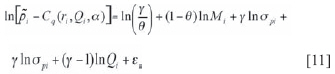
where the income of the season is determined by the average price and the production. 

S = σ _p Q                                                                           [8]

where σ_p is the standard deviation of prices.

Assuming that the producer maximizes his utility derived from wealth, we can write the producers` optimization problem as Equation [9]:

The first order condition (FOC) for this function is:

where C_q is marginal cost. If γ = 0, that is, if the producer were neutral to risk, Equation [10] would simplify to “price equals marginal cost” condition.  

Equation [10] proposes that the difference between the average price and marginal cost (left side of the equation), can be explained by the risk preferences of the producer. To estimate Equation [10], we apply natural logarithm, obtaining Equation [11]:

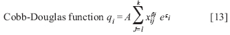
The sub-index i denotes the ith observation, ε_i corresponds to the estimation error, and α represents the technological parameters of the cost function, whose form is assumed to be known.

Equation [11] considers the differential between average price and marginal cost as an independent variable, that is, the risk premium that the producer expects, given his risk preferences. The right-hand side of Equation [11] corresponds to a production function whose formal function shall be defined based on empirical estimations. This equation allows estimating the parameters θ and γ to identify the risk preferences of raspberry producers.

Saha et al. (1994b) conclude that for a more efficient estimation, the technological and risk preferences parameters should be estimated jointly. 

For the production function, two functional forms were estimated: quadratic and Cobb-Douglas.

Quadratic function                   

q_i = β₀ + β₁ x² + β₂ x² _i2 +.... +β_n x² _in + ε_i                  [12]

Cobb-Douglas function

Where the sub-index i indicates the ith individual and ε_i is the error term of the equation. The x_ij are explanatory variables that should be sought among a wide set. In the case of the Cobb-Douglas function, the values of the β_j parameters reflect the contribution of production factors in the profit and А represents exogenous technological progress.  

Data source

The data for estimating the equations was gathered through a survey applied to a sample of 62 producers in the Bío Bío Region. The survey was applied during the months of March and April of 2007. The sample was taken in the three counties of the region that have the highest concentration of raspberry producers. The information with regard to the raspberry producers and the total surface area planted at county level was provided by Jorge Vargas (2007), in charge of Good Agricultural Practices, Servicio Agrícola Ganadero (SAG), personal communication. The number of individuals surveyed in each county was: Coihueco (43 surveys), San Carlos (3 surveys) and Ñiquén (16 surveys). The information gathered was the following: amount of fertilizer used (F), fuel used (E), labor contracted for harvesting (T), area planted with raspberry per producer (size), number of years that the producer has cultivated raspberries (experience), production of raspberries (Q), gross income (M), average selling  price of raspberries (), price variation (σ_p) and marginal production cost (C_q). The information gathered was from the 2006-2007 season. The estimations were made with the econometric program Eviews 5.1 (Quantitative Micro Software, 2004).

RESULTS AND DISCUSSION

The sample used is of small producers, whose data presents a high variability (Table 1). The average area of the raspberry crop was 0.6 ha. Total income per hectare fluctuates between $23000 and $4760000, with an average earning of $1401536. This variability in incomes is explained by the variability of surface planted, production costs and productivity. The average yield was 8270 kg ha^-1, with a range between 1467 and 24000 kg ha^-1.   

Table 1. Estadística descriptiva de las variables utilizadas en el modelo. Abril 2007

Table 1. Descriptive statistics of the variables used in the model. April 2007

                      Valor del dólar a la fecha del estudio: 1 US$ = 532 $ Chilenos

In terms of the producers` characteristics, the average age was 51 years, and the majority of them have a low level of schooling: 6.4% were illiterate, and 61.3% had only basic level education, either partial or completed. The surveys were taken to the member of the family responsible of the raspberry orchard, in which, 55% of the sample was male and 45% female. As well, the survey subjects were asked about their main occupation. Only 55% of the sample declared themselves as farmers. A high percentage, 37% of the total sample, declared housewife as their main occupation (which correspond to 82% of the total of women). Table 1 presents the mean, minimum and maximum values of the variables of the system of estimated equations.  

Production function election

Two functional forms were evaluated: quadratic and Cobb-Douglas. The variables of the final model were chosen from among the following: fertilizer (total kg/number of hectares), fuel (total liters/number of hectares), work (boxes harvested/number of hectares), experience (number of years that the producer has worked in raspberry production on the farm), surface area planted and a dichotomous variable for technical advisory. Based on this estimation, the non significant variables were eliminated. The results showed that the Cobb-Douglas functional form adjust best to the data. Table 2 shows that while the quadratic function exhibits a greater coefficient of multiple determination (R²), the test for model specification, Akaike Information Criteria, Schwarz criteria and Log Likelihood, indicated a better adjustment of the Cobb-Douglas function. The model does not present heteroscedasticity or self-correlation, and the errors exhibit a normal distribution.  

Table 2. Resultados de criterios de elección para la función de producción.

Table 2. Results of the selection criteria for the production function.

R²: Multiple determination coefficient.
Adjusted R²: Multiple determination coefficient adjusted by degrees of freedom.

Estimation of risk preferences

The risk preferences parameters, θ and γ, were estimated through Equation [11] and the production function represented in Equation [13]. The estimation of this system of equations was done through three alternative methods in order to identify the most efficient: Ordinary Least Squares, Seemingly Unrelated Regression (SUR) and Full Information Maximum Likelihood (FIML). The method of ordinary least squares allows for estimating separately the parameters of Equations [11] and [13]. In the case of SUR, the joint estimation is characterized by assuming the presence of heteroscedasticity and contemporary correlation among the errors of the equations. This method is recommended for systems of equations where the independent variables are totally exogenous to the system, which in this case represents an inconvenience given that it has two equations and only one totally independent exogenous variable. Finally the FIML method is designed for both lineal and non-lineal systems, being the basic assumption of this method that the errors have a joint normal distribution (Quantitative Micro Software, 2004).  

Analyzing the results under the three methods, it is possible to conclude that the estimations by SUR and FIML are not more efficient than the ordinary least square estimation, such as suggested by Saha et al. (1946), given that the sum of squared errors of the estimation is not significantly reduced with the joint estimation. As well, it was possible to verify that the errors of Equation [11] do not have a normal distribution, so it does not comply with the supposition of joint normality for the errors, considered in the FIML estimation. Table 3 summarizes the results of the estimation by ordinary least squares of Equations [11] and [13].

Table 3. Parámetros estimados de la condición de primer orden (CPO) y función de producción.

Table 3. Estimated parameters for the first order condition (FOC) and production function.

 * Significance at 5%; ** Significance at 1%.

θ and γ are the parameters that determine the degree risk avoidance; Ln fertilizer is the natural logarithm of kg ha^-1 of fertilizer; Ln experience is the natural logarithm of the number of years of experience in the cultivation of raspberries; and Ln size is the natural logarithm of planted hectares.

In the production function, the variables experience, size of planted area and quantity of fertilizer used resulted significant (Table 3). According to the results, the experience acquired in the cultivation of raspberries measured by the number of years that the producers has been involved in cultivating this berry, allows for explaining differences in the levels of production among producers. According to these results, two additional years of experience implies an average increase in production of 1.21 kg ha^-1. On the other hand, an increase of 2 kg of fertilizer allows for increasing production by 1.09 kg ha^-1, assuming an average yield of 8270 kg ha^-1 (Table 1).

Another relevant variable is the size of the total surface planted with raspberry. It was observed that the size variable had a negative effect on raspberries production. One explanation could be that some of these large scale producers, with greater possibilities of investment, enter in the fresh market production, motivated by important price differentials, privileging quality over quantity.  

The estimations of the parameters θ and γ indicate that on average raspberry producers are averse to risks, and present an absolute and relative increasing aversion. This is deduced from the values of the parameters, for which γ > 0, θ < 1 and θ < γ. In other words, as the level of risk of an activity increases, producers are more adverse to risk. On the other hand, the relative increasing aversion indicates that to the extent that producers have a greater level of income, they tend to be more risk averse. These results imply, for example, that producers are increasingly more reticent to accept innovations or crops that involve assuming greater risks than those that they are already accepting. Besides, it implies that producers who receive higher incomes will be more unwilling to accept these innovations or crops with higher risk than those they are currently accepting.  

The values of aversion obtained in this study are relatively low compared to estimations done by Saha (1997) and Isik and Khanna (2003), who used the flexible utility function of Saha (1997) (Table 4).

Table 4. Comparación de parámetros de aversión al riesgo con diferentes estudios.

Table 4. Comparison of risk aversion parameters with different studies. 

* Significance at 5%; ** Significance at 1%.
¹The values of the parameters reported by Saha (1997) correspond to a sub-sample of the smallest scale producers.

Saha (1997) applied the flexible utility function to estimate risk preferences for a set of 15 wheat producers in the state of Kansas, USA, from whom he obtained information for four years, totaling 60 observations. Later, the sample was sub-divided into two sub-samples with the goal of evaluating the scale of the producers on the structure of risk preferences. The results of Saha (1997) indicated that agricultural producers of a lower scale are less adverse to risk (lower estimated value for the γ parameter). The parameters reported in Table 4 were for the smaller producers.

On the other hand, Isik and Khanna (2003) estimated the system of compound equations for the first order condition and for a quadratic production function. They used a non- linear least squares in three stages estimation method, given that the authors considered the system of equations as a simultaneous problem. They used 198 observations that corresponded to two seasons. The information was gathered from corn producers in the state of Illinois, USA.

The estimated degree of risk aversion in this study was γ = 0.10, while those estimated by Saha (1997) and Isik and Khanna (2003) are 1.9 and 1.6, respectively; equally important differences can be observed in the estimation of the θ parameter. These differences can be attributed to several reasons, not ruling out that effectively the group used in the present study is less averse to risk. The first explanation is that the producers included in the samples used in the other studies are of a larger scale, which in a scenario of absolute and relative increasing aversion would explain the difference very clearly (the articles of Saha (1997) and Isik and Khanna (2003) do not make explicit the scale of the producers considered). The second explanation is related to the information used in the estimations. In the article of Saha (1997) expectations about future prices are considered and in Isik and Khanna (2003) information about fertility and soil depth is used. These differences in the information used, as well as variables of the environment associated with the USA could explain the differences in the values of the estimated parameters.

Hypothesis test of the estimated parameters  

There are several hypotheses about the coefficients that are appropriate to test before making an analysis of them. The results of the hypothesis tests shown in Table 5 allow for concluding, the following: a) The hypothesis of constant returns to scale (production function) is rejected, with 99% confidence; b) The hypothesis of  a lineal form for the utility function (Equation [4]) is rejected, with 99% confidence; c) the hypothesis of absolute constant aversion to risk is rejected with 99% confidence; d) There is not sufficient statistical evidence to reject relative constant aversion to risk; and e) The hypothesis of neutrality to risk is rejected, with 94% confidence.

Table 5. Resultados de las pruebas de hipótesis sobre parámetros del modelo.

Table 5. Results of tests of hypothesis of the parameters of the model.

⁽¹⁾ To do hypothesis test with simultaneous restrictions, as the second hypothesis, Eviews 5.1 reports the normalized coefficients for each of the restrictions. The first coefficient is θ and the second is γ.

These tests of hypothesis allow for verifying that returns to scale are decreasing, given that the sum of β₂ + β₃ + β₄ is equal to 0.18, that is, if we double the quantities of factors included in the production function, the resulting output would increase by less than double. In other words, the raspberry producer who wants to double his production would have to more than double the quantity of fertilizer and experience. As well, the results show that economic agents are not neutral to risk and that they are not indifferent to distinct levels of risk. These results put into question one of the most common assumptions in the evaluation of both private and public initiatives, given that it is demonstrated that agents are not neutral to risk and that producers decisions are sensitive to the levels of risk of the alternatives analyzed.

CONCLUSIONS

The results of the estimations indicated that small-scale raspberry producers in the Bío-Bío Region are risk averse (γ > 0), that they have an increasing absolute (θ < 1) and relative aversion (θ < γ). That is, the risk aversion increases as the risk of an activity is greater and the income of the producer is higher.

The results of the estimation of the raspberry production using a Cobb-Douglas function reveals that the returns to scale are decreasing (returns to scale = 0.18) and that the relevant factors in determining yield are the experience of the producer, the size of the plantation and fertilizers dosage.  

LITERATURE CITED

• Abadi, A.K., D.J. Pannell, and M.P. Burton. 2005. Risk, uncertainty, and learning in adoption of a crop innovation. Agric. Econ. 33:1-9.
• Arrow, K.J. 1964. The role of securities in the optimal allocation of risk bearing. Rev. Econ. Stud. 31(2):91-96.
• Isik, M., and M. Khanna. 2003. Stochastic technology, risk preferences, and adoption of site-specific technologies. Am. J. Agric. Econ. 85:305-17.
• Kahneman, D., and A. Tversky. 1979. Prospect theory: An analysis of decision under risk. Econometrica 47:263-92.
• Lusk, J.L., and K.H. Coble. 2005. Risk perceptions, risk preference, and acceptance of risky food Am. J. Agric. Econ. 87:393-405.
• Markowitz, H.M. 1959. Portfolio selection: Efficient diversification of investment. 344 p. John Wiley & Sons, New York, USA.
• Meyer, J. 1987. Two-moment decision models and expected utility maximization. Am. Econ. Rev. 77:421-30.
• Pratt, J.W. 1964. Risk aversion in the small and in the large. Econometrica 32(1-2):122-136.
• Quantitative Micro Software. 2004. Eviews 5.1. User guide. Quantitative Micro Software. Irvine, California, USA.
• Saha, A. 1993. Expo-Power Utility: A ‘flexible’ form for absolute and relative risk aversion. Am. J. Agric. Econ. 75:905-13.
• Saha, A. 1997. Risk preference estimation in the nonlinear mean standard deviation approach. Econ. Inquiry 35:770-82.
• Saha, A., H.A. Love, and R. Schwart. 1994a. Adoption of emerging technologies under output uncertainty. Am. J. Agric. Econ. 76:836-46. 
• Saha, A., R. Shumway, and H. Talpaz. 1994b. Joint estimation of risk preference structure and technology using Expo-Power Utility. Am. J. Agric. Econ. 76:173-184.
• Tobin, J. 1958. Liquidity preferences as behavior towards risk. Rev. Econ. Stud. 25:65-86.
• Von Neumann, J., and O. Morgenstern. 1944. Theory of games and economic behaviour. 776 p. Princeton University Press, Princeton, UK.

Copyright 2008 - Instituto de Investigaciones Agropecuarias, INIA (Chile).