 |
| About Bioline | All Journals | Testimonials | Membership | News |
|
||||||
|
||||||
Chilean Journal of Agricultural Research (formerly Agricultura Técnica), Vol. 68, No. 4, Oct-Dec, 2008, pp. 360-367 Research Technological change and technical efficiency for dairy farms in three southern countries of South America Cambio tecnológico y eficiencia técnica en predios lecheros de tres países de Sudamérica. Boris E. Bravo-Ureta[1], Víctor H. Moreira [2]*, Amilcar A. Arzubi[3], Ernesto D. Schilder[4], Jorge Álvarez[5], and Carlos Molina5 [1] University of Connecticut, Department of
Agricultural and Resource Economics, Storrs, 06269, Connecticut, USA. E-mail: boris.bravoureta@uconn.edu. Received: 11 October 2007. Code Number: cj08038 ABSTRACT The progressive liberalization of agricultural markets, along with the threat that imported products can pose to local producers, reveals the importance of productivity growth as a mechanism to improve competitiveness. Technical efficiency measurement is the most studied component of productivity because it can help to generate valuable information for policy formulation and farm level decisions focused on the improvement of farm performance. This study uses unbalanced panel data sets for dairy farms from Argentina, Chile and Uruguay, to estimate stochastic production frontier models. These frontiers are then used to estimate economies of size, technological change and technical efficiency. All estimations are based on the Battese and Coelli (1992) model, which is widely used in empirical productivity studies. The models for all three countries exhibit increasing returns to scale, which suggests that the dairy farms in the samples are operating at a sub-optimal size. The average annual rate of technological change for Argentina was 0.9%, for Chile 2.6% and for Uruguay 6.9%, while average technical efficiency was 87.0%, 84.9% and 81.1%, respectively. Keywords: stochastic frontiers, dairy farms, Argentina, Chile, Uruguay. RESUMEN La liberalización progresiva de los mercados agrícolas, junto a la amenaza que implica para productores nacionales la competencia de productos importados, dejan en claro la relevancia del incremento en la productividad como un elemento para mejorar la competitividad. La medición de la eficiencia técnica es uno de los componentes de la productividad más estudiados, debido a que proporciona información valiosa al momento de formular políticas y tomar decisiones destinadas a mejorar la administración predial. Este trabajo utiliza datos de panel desbalanceados de predios lecheros provenientes de Argentina, Chile y Uruguay, para estimar fronteras estocásticas de producción. Luego estas fronteras se usaron para analizar economías de tamaño, tasas de cambio tecnológico y eficiencia técnica. En todas las estimaciones se empleó el modelo de Battese y Coelli (1992), ampliamente usado en la literatura de productividad. Los modelos para los tres países exhiben economías de escala crecientes, lo que implica que los predios en las muestras operan a un tamaño sub-óptimo. La tasa promedio anual de cambio tecnológico fue 0,9% para Argentina, 2,6% para Chile y 6,9% para Uruguay mientras que la eficiencia técnica media fue igual a 87,0%, 84,9% y 81,1%, respectivamente. Palabras clave: fronteras estocásticas, predios lecheros, Argentina, Chile, Uruguay. INTRODUCTION Beginning with the Uruguay Round of the World Trade Organization (WTO), which opened in 1997, the multilateral liberalization of agricultural markets has been an important goal that has been strengthened by the reduction of protective tariffs in many countries (Hanrahan and Schnepf, 2005). The same authors point out that another element that helps to project a scenario of increasing liberalization of agricultural markets is the leading role that this sector played in the failed Doha Round in Qatar, which began in 2001. The opening up of trade has brought the increased competition of imported products in many markets, and it can be expected that new agricultural products will be incorporated into this process of liberalization. In this new scenario, the dairy sector plays a very important role in all the discussions about the liberalization of markets, fundamentally because of the high level of protection in many countries, and also because it is expected that the milk sector will experiment significant expansion globally, especially in Asia, North Africa, the Middle East, Central America and the Russian Federation (FAO, 2003; Blayney and Gehlhar, 2005; European Commission, 2005). The progressive liberalization of agricultural markets, and the threat that the competition of imported products represents for local producers reveals the importance of improving productivity as a key factor to counteract pressures from countries that present greater competitiveness (Pinstrup-Andersen, 2002; Ruttan, 2002). An example that illustrates this process is the case of New Zealand, where the unilateral dismantling of agricultural subsidies has been accompanied by significant increases in farm efficiency and in total factor productivity at the national level (Sandrey and Scobie, 1994; Evans et al., 1996; Paul et al., 2000; ABARE, 2006). Today, New Zealand is the major exporter of milk products in the world (Blayney and Gehlhar, 2005). To achieve significant increases in productivity and competitiveness, policies are required that encourage the adoption of new technologies, as well as measures that promote the efficient use of existing technologies. It is also necessary that policy makers, producers and agricultural extensionists have access to empirical studies that allow them to elucidate the effects of different factors that influence increases in productivity (Russell and Young, 1983; Kalirajan, 1984). Despite the importance of this topic, there are only a few specialized studies that consider the case of the Southern Cone countries of South America. Consequently, the objective of this paper was to analyze the level of technical efficiency (TE) at the micro-economic level (farm), considering samples of dairy farms in Argentina, Chile and Uruguay. In addition, technological change (TC) and economies of size (EOS) were analyzed for the three samples. MATERIALS AND METHODS Stochastic production frontier To achieve the proposed objectives, stochastic production frontiers (SPF) were estimated, using unbalanced panel data. Frontier models can be classified into two basic types: parametric and non-parametric. Parametric frontiers require the specification of a particular functional form and can be classified as deterministic and stochastic. The deterministic model assumes that any deviation from the frontier is due to inefficiency, while the stochastic incorporates statistical noise. In this respect, in the case of deterministic frontiers, any measurement error and any other source of stochastic variation in the dependent variable is attributed to inefficiency, making the estimations of TE sensitive to extreme values (Greene, 1993). On the other had, the SPF resolves the problem of extreme values incorporating a compound error with a two-sided symmetrical term and a one-sided component. The latter reflects inefficiency, while the two-sided error captures random effects outside the control of the production unit. The production frontier used here follows the structure of Battese and Coelli (1992), which has become very popular in recent years. In 1995 these authors published an extension of the original model, which is typically used when there are data that can be used to explain the variation in TE (Battese and Coelli, 1995). However, in the present study, such data were not available. In accordance with Battese and Coelli (1992), the SPF can be represented as: Yit = exp(xitβ + Vit – Uit) [1] where Yit is the output of the i-th farm in the
t-th time period; xit is a vector (1 x K)of
inputs and other explanatory variables for the i-th farm in the t-th time
period; β is a
vector (K x 1) of the unknown parameters to be estimated; Vit
is the random error, which is supposed to have a normal distribution with mean
zero and constant variance ( Following Battese and Coelli (1992), Uit can be defined as: Uit = {exp[-η(t – T)]} Ui [2] where η is an unknown scalar to be
estimated, t is the time period analyzed and T is the total
number of periods. TE increases, remains constant or decreases with time when η > 0, η = 0 or η < 0, respectively. The Uit
term can have different specifications and the most popular are the
non-negative distribution of a truncated normal with an average m and a constant variance (Ui
~ iid/N(μ, TE for the i-th farm is given by: TE = exp(-Ui) [3] where U is specified in equations [1] and [2]. The TE for each farm is calculated by using the conditional expectation of -Ui (exp(-Ui)), given the compound error term (V-U) (Jondrow et al., 1982; Battese and Coelli, 1988). All these calculations were done using the software FRONTIER 4.1, which provides maximum likelihood estimates for the parameters of the stochastic frontier model (Coelli, 1996). FRONTIER 4.1 is a program that is often used in estimations of stochastic frontiers and its distribution is free (Sena, 1999), which is not the case with other alternative programs (e.g., LIMDEP, STATA). Considering the specification
indicated above, the null hypothesis that technical inefficiency is not present
in the model was tested. This is equivalent to saying that γ = 0,
taking into account that this parameter corresponds to the ratio between the variance
of the one-sided error ( Data and empirical model Descriptive statistics for the data used in this analysis are presented in Table 1. The data from Argentina came from a sample of dairy farms located in the Abasto Sur basin, in Buenos Aires Province. The data was collected by researchers from the Universidad de Lomas de Zamora in Buenos Aires, incorporating three agricultural periods (1997-1998, 1999-2000 and 2001-2002), and included 46 dairy farms with a total of 82 observations. The data from the Chilean sample came from 48 farms of small milk producers belonging to the Farm Management Center of Paillaco, Valdivia, located in the south of the country in the communities of Paillaco, Los Lagos and Futrono, and covers the agricultural years of 1996-1997, 1998-1999, 1999-2000, 2000-2001 and 2001-2002, with a total of 92 observations. The Uruguayan data, collected by researchers from the Universidad de la República, in Montevideo, cover four agricultural years (1999-2000, 2000-2001, 2001-2002 and 2002-2003) and include 70 dairy farms and a total of 147 observations. It is evident that all three data sets are unbalanced panels. All variables expressed in monetary values were available in nominal dollars for each period and country. The nominal dollars were adjusted according to the purchasing power of each country (Argentina, Chile or Uruguay) in comparison to the United States, using the Consumer Price Index (CPI) of each country. This was done by multiplying the nominal dollars by the CPI of the United States, and subsequently dividing it by the specific CPI of each country, for each one of the periods considered. All the adjusted variables are then converted to real dollars using the period of July 2004 – June 2005 as the base. Table 1. Descriptive statistics of dairy farm data for Argentina, Chile and Uruguay
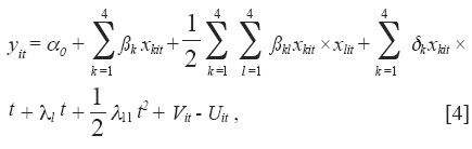
a SD: standard deviation; b US$, the reference year is July 2004-June, 2005 or 2004-2005; c Corresponds to total farms. Three separate SPF models were estimated, one for each country, using a translog (TL) specification. This model can be represented as:
where the sub-indexes k represent the k-th explanatory variable, i reflects a specific farm, t is a tendency variable to capture TC, and the sub-index j, which indicates the country, is omitted to simplify the exposition. The dependent variable (y) is the natural logarithm for annual output per farm, measured in liters. The explanatory variables, also expressed in natural logarithms, are the following: average number of cows per dairy farm (CO); labor, measured in equivalent workers (LB); purchased feed (FD) including concentrate feed, hay, minerals and all the costs associated with the production of hay, ensilage and grass; and veterinary input costs (VE). The definition of t as a tendency variable that captures TC is modified with each data set. In this manner, the value of t for Argentina is 1 = 1997-1998, 3 = 1999-2000, and 5 = 2001-2002; for Chile 1 = 1996-1997, 3 = 1998-1999, 4 = 1999-2000, 5 = 2000-2001, and 6 = 2001-2002; and for Uruguay 1 = 1999-2000, 2 = 2000-2001, 3 = 2001-2002 and 4 = 2002-2003. The random terms Vit and Uit are the same as were already defined in Equations [1] and [2], and the Greek letters represent the parameters to be estimated. As is common practice in the TL models, all variables are expressed as deviations from the geometric mean, which makes it possible to interpret the linear coefficients directly as partial elasticities of production. RESULTS AND DISCUSSION Different specifications of the stochastic frontier were estimated for the three countries, with the objective of determining the most consistent model for the available data. The preliminary analysis revealed that the TL functional form is superior to the Cobb-Douglas, which is consistent with the production frontier literature (Coelli et al., 2005; Bravo-Ureta et al., 2007). The term that captures TE follows a half-normal distribution, and TE is statistically significant and constant over time. Consequently, the analysis developed from here on is limited to the results from the model with these predominant characteristics. More details regarding the procedures used for model selection can be found in Moreira (2006). In the model for Argentina the linear parameters were highly significant, with the exception of the coefficient for the time trend t. The parameter for t2 (time squared) was positive and significant, while the only significant parameters for the interaction terms were those for t and VE (veterinary inputs) (Table 2). The coefficient for CO (cows) was the most important among the partial elasticities, which implies that a percentage change in the number of cows would have a greater influence on milk production than a similar change in any other input. These results are consistent with many other studies, including Kumbhakar et al.(1991), Arias and Álvarez (1993), Heshmati and Kumbhakar (1994), Ahmad and Bravo-Ureta (1996), Jaforullah and Devlin (1996), Cuesta (2000), Lawson et al.(2004a; 2004b), and Moreira et al.(2006). Table 2. Parameter estimates for translog production frontiers of dairy farms in Argentina, Chile and Uruguaya
***
1% of the level of significance. ** 5% of the level of significance, *10% of
the level of significance. The model for Chile also presented highly significant first order parameters, with the exception of LB (labor) and t (Table 2). Most of the comments made for Argentina are also valid for Chile, except for the parameter for t2, which was negative and significant and the parameters for the interaction between t and the other inputs that were not significant. The results in Table 2 also show that the first order parameters for the Uruguayan model were highly significant, with the exception of LB. The t2 parameter was not significant and, as in the Chilean case, none of the parameters for the interaction between t and the other inputs were significant. The function coefficient is the indicator commonly used to measure economies of size (EOS) in primal models, such as the SPF being used here. For the model presented in Equation [4] the function coefficient is equal to:
Given that the data is normalized by
the geometric mean, the function coefficient calculated at this mean is equal
to the sum of the linear parameters ( Table 3. Economies of size (EOS) of Argentinean, Chilean and Uruguayan dairy farms
Another important dimension of the productive structure, which can be analyzed, based on the econometric estimations of a production frontier with panel data, is TC. For the TL model in Equation [4] the expression for TC is equal to:
The annual rate of TC, at the geometric mean, is equal to the linear coefficient of the tendency variable (λ1) which in this case is 0.9, 2.6 and 6.9% for Argentina, Chile and Uruguay, respectively. To examine the variation over time, Table 4 provides the annual rate of TC for each country according to the available information. It can be observed that for Argentina there is a very low and negative annual rate between 1997-1998 and 1998-1999 (-1.1%), which then rose between 1999-2000 and 2000-2001 (2.1%). In the case of Chile, there was a clear deterioration between 1996-1997 and 1997-1998 (5.5%) and 2000-2001 and 2001-2002 (-4.4%). In the case of Uruguay, an important TC rate was observed during the period under analysis, which experienced a reduction between 1999-2000 and 2000-2001 (11.9%) and 2000-2001 and 2001-2002 (8.0%), and then an increase in 2001-2002 and 2002-2003 (13.6%). Table 4. Technological change (TC) for Argentinean, Chilean and Uruguayan dairy farms
a Base year for Argentina is 1997-1998; b Base year for Chile is 1996-1997; c Base year for Uruguay is 1999-2000; d na: not available; e The results of the previously period were used because of lack of information. Table 5 shows descriptive statistics for the TE measures for each country. The average TE for Argentina was 87.0% with a minimum of 69.1% and a maximum of 97.9%. The average in the case of Chile was 84.9% with extremes of 64.4 and 94.8%. The statistics for Uruguay show an average of 81.1% with a variation between 49.3 and 97.1%. Several studies of dairy farms that use the stochastic frontier model have TEs close to the results of this research, as was reported by Moreira (2006). Table 5. Technical efficiency (TE) of Argentinean, Chilean and Uruguayan dairy farms
It is important to note that the different indicators of productivity reported in this paper were calculated individually for each country and their respective production frontiers, so they are not directly comparable. In order to compare these indicators it is necessary to formally analyze whether the samples have access to the same level of technology. This idea is the basis of the meta-frontier production function, an approach recently developed by Battese et al.(2004) and refined by O’Donnell et al.(2008). CONCLUSIONS This study used unbalanced panel data for dairy farms from Argentina, Chile and Uruguay to estimate stochastic production frontiers. These frontiers were used to evaluate economies of size (EOS), rates of technological change (TC) and technical efficiency (TE). In the preliminary analysis it was shown that the translog functional form (TL) is superior to the Cobb-Douglas. The term that captures TE follows a half-normal distribution and is statistically significant and constant over time, presenting mean values of 87.0, 84.9 and 81.1% for Argentina, Chile and Uruguay, respectively. This result makes evident that the dairy farmers included in the sample of the three countries could increase their milk production by 13.0, 15.1 and 18.9%, respectively, without increasing the use of inputs. Average TC was 0.9% for Argentina, 2.6% for Chile and 6.9% for Uruguay. Finally, increasing EOS were found, which implies that the farms in the sample operate at a sub-optimal size. LITERATURE CITED
Copyright 2008 - Instituto de Investigaciones Agropecuarias, INIA (Chile). The following images related to this document are available:Photo images[cj08038t4.jpg] [cj08038t3.jpg] [cj08038t2.jpg] [cj08038t1.jpg] [cj08038t5.jpg] | |||||||||||||||||||||||||||||||||||||||||||||||||||||||||||||||||||||||||||||||||||||||||||||||||||||||||||||||||||||||||||||||||||||||||||||||||||||||||||||||||||||||||||||||||||||||||||||||||||||||||||||||||||||||||||||||||||||||||||||||||||||||||||||||||||||||||||||||||||||||||||||||||||||||||||||||||||||||||||||||||||||||||||||||||||||||||||||||||||||||||||||||||||||||||||||||||||||||||||||||||||||||||||||||||||||||||||||||||||||||||||||||||||||||||||||||||||||||||||||||||||||||||||||||||||||||||||||||||||||||||||||||||||||||||||||||||||||||||||||||||||||||||||||||||||||||||||||||||||||||||||||||||||||||||
| |||||||||
 , [4]
, [4]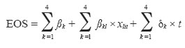 [5]
[5]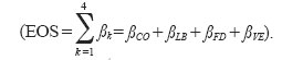 ). Consequently, the samples for the three
countries reveal the presence of EOS, the largest being for Argentina (1.231), followed by Chile (1.100) and then by Uruguay (1.068). To obtain a broader vision
of the behavior of EOS, Table 3 shows the function coefficient for four
groups of farms of different size. The groups were defined according to the
number of cows per quartile for each country. For Chile and Argentina, EOS decreased monotonically as the average number of cows rose. The data suggests that
the average cost curve for Argentina is L-shaped, while that of Chile is U-shaped. In the case of Uruguay, EOS increases monotonically with the number of
cows and this insinuates an average cost curve with a negative slope.
). Consequently, the samples for the three
countries reveal the presence of EOS, the largest being for Argentina (1.231), followed by Chile (1.100) and then by Uruguay (1.068). To obtain a broader vision
of the behavior of EOS, Table 3 shows the function coefficient for four
groups of farms of different size. The groups were defined according to the
number of cows per quartile for each country. For Chile and Argentina, EOS decreased monotonically as the average number of cows rose. The data suggests that
the average cost curve for Argentina is L-shaped, while that of Chile is U-shaped. In the case of Uruguay, EOS increases monotonically with the number of
cows and this insinuates an average cost curve with a negative slope.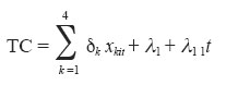 [6]
[6]