 |
| About Bioline | All Journals | Testimonials | Membership | News |
|
||||||
|
||||||
Chilean Journal of Agricultural Research (formerly Agricultura Técnica), Vol. 68, No. 4, Oct-Dec, 2008, pp. 368-379 Research Export behaviour in the Chilean agribusiness and food processing industry Comportamiento exportador de las empresas chilenas, agrocomerciales y procesadoras de alimentos. Rodrigo Echeverría[1]*, and Munisamy Gopinath[2] [1] Universidad Austral de Chile, Instituto de
Economía Agraria, Campus Isla Teja, Valdivia, Chile. E-mail: rodrigoecheverria@uach.cl
* Corresponding author. Received:
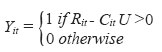
20 November 2007. Code Number: cj08039 ABSTRACT This paper analyzes the export-behavior of Chilean agribusiness and food processing firms and the relative importance of firm-specific and geographic characteristics in this behavior. Using firm level data and regional geographic indicators, a dynamic model was used to study the export decisions and the export intensity of three industries: processing fish, processing fruits and vegetables, and wine production. Results showed that determinants of exporting behavior vary among the three industries, except the effect of sunk costs, which strongly impacts the export decisions of all analyzed industries. This implies that firms with prior export experience will have higher probability of exporting in the future. Foreign ownership positively impacts the export decision of the two processing industries. Thus, firms belonging to these industries that wish to increase the probability of being an exporter should be encouraged to have a partnership with a foreign company or investor. The export intensity is positively influenced by foreign ownership in the fruit and vegetables processing and wine industries. As in the case of the export decision of firms, foreign participation helps increase the scale of exports. In general, firm-specific characteristics significantly impact the export behavior in Chilean agribusiness and processed food industries, while the contribution of geography attributes appears mixed. Key words: agricultural trade, export decision, export intensity, geography. RESUMEN Este artículo analiza el comportamiento exportador de las empresas chilenas agroindustriales y procesadoras de alimentos y la importancia relativa que las características geográficas y específicas de las empresas tienen en este comportamiento exportador. Con datos a nivel de empresas e indicadores geográficos regionales, se utilizó un modelo dinámico para estudiar la decisión y la intensidad exportadora de tres industrias: industria procesadora de pescados, industria procesadora de frutas y hortalizas, e industria productora de vinos. Los resultados indican que las determinantes del comportamiento exportador varían entre las tres industrias, excepto el efecto de los costos hundidos, los cuales impactan fuertemente la decisión de exportar de todas las industrias analizadas. Esto implica que las empresas con experiencia exportadora previa tendrán mayores probabilidades de exportar en el futuro. La propiedad extranjera impacta positivamente la decisión de exportar de las dos industrias procesadoras. Así, las empresas de estas industrias que deseen aumentar sus probabilidades de llegar a ser exportadoras, deberían tratar de asociarse con empresas o inversionistas extranjeros. La intensidad de exportación está positivamente influenciada por la propiedad extranjera en la industria procesadora de frutas y hortalizas, y en la industria vitivinícola. Así como en el caso de la decisión de exportar, la participación extranjera ayuda a incrementar la escala de las exportaciones. En general, las características específicas asociadas a las empresas impactan significativamente el comportamiento exportador de las agroindustrias e industrias chilenas procesadoras de alimentos, mientras que la contribución de los atributos geográficos no es del todo clara. Palabras clave: comercio agrícola, decisión de exportar, intensidad de exportación, geografía. INTRODUCTION The positive correlation between exports and economic growth has led to a flurry of export promotion activities by developed- and developing-country governments (Frankel and Romer, 1999; Giles and Williams, 2000; Herzer et al., 2006). As a result of the Uruguay/Doha round of the World Trade Organization (WTO) negotiations (Hoda and Gulati, 2008), export subsidies are being phased out, and many of these promotional activities are aimed at helping firms/producers overcome informational and knowledge asymmetries, and credit and exchange rate risks. Yet the factors that underlie a firm’s decision to export, continue to export or exit a foreign market have received limited attention until recently (Wagner, 2007). Part of the problem is that the export-led growth theory has been mostly macroeconomic in design and applications. The small number of firm-level export studies reflects problems of data availability, as well as the limited understanding of the characteristics of exporting firms, which are critical to the design of an effective policy to encourage trade participation (Roberts and Tybout, 1997; Bernard and Jensen, 1999; Helpman et al., 2004). Since the seminal contributions of Bernard and Jensen (1995) and Aw and Hwang (1995), several studies have found that exporters perform better than non-exporters. In general, exporting firms are larger, more capital intensive, pay higher wages, hire more skilled workers, and, most importantly, they are more productive than the non-exporters (Clerides et al., 1998; Bernard and Jensen, 1999; 2004b; Girma et al., 2004; Bernard et al., 2007). However, the economic-geography literature highlights the important effect of locational characteristics on firms’ productivity and thus, performance (Krugman, 1991; Aitken et al., 1997). The latter studies have found that exporters tend to geographically concentrate, suggesting that geography may play an important role in firms’ export behavior. Most studies include geographic characteristics using categorical variables such as regional or provincial indicators (Roberts and Tybout, 1997; Limao and Venables, 2001; Bernard and Jensen, 2004a). Others, e.g., Venables (2005), find this simple representation of locational forces inadequate, since geography and exports figure prominently in factors determining spatial income inequality within many developing countries. In some industries, particularly those related to natural resources, geography may play a dominant role in the location of enterprises. As a consequence, production of these industries could be restricted mostly by geography, and firm-specific characteristics may be less important. Indeed agribusiness and food processing industries appear to fit the above hypothesis well. For example, as production of farms is conditioned by geographical factors such as weather or soil type, it is not clear whether the export activity of related processing firms -agribusiness- is determined mostly by geographical factors or firm-specific characteristics, as in export-decision studies. Thus, the purpose of this study was to investigate the relative importance of firm-specific and geographic characteristics in the export behavior of firms in the Chilean agribusiness and food processing industries. MATERIALS AND METHODS Model The empirical framework for firms’ export behavior in this study is based on the dynamic model with sunk entry/exit costs proposed by Roberts and Tybout (1997). Sunk costs include those on collecting information about foreign markets, creating and maintaining marketing networks, and negotiating and enforcing new contracts (Basile, 2001). Note that many of these costs cannot be recovered if the firm decides to stop selling abroad, i.e., exit costs. Hence, Roberts and Tybout (1997) and Bernard and Jensen (2004b) model the decision to export, or continue to export or exit a foreign market as a function of sunk entry/exit costs. Let Ri(p, Si) denote additional revenue from exporting of the i-th firm, i = 1, 2,…, N, given prices p and firm-specific factors Si, including size, productivity, ownership structure and locational factors affecting firm i. At time t, a firm exports, Yit = 1, if export revenues exceed costs of production, Cit, and any sunk costs of exporting, U:
In order to identify a firm’s probability of exporting, Equation [1] can be estimated as a binary (discrete) choice using a non-structural approach:
where the vector Xit
includes the firm-specific characteristics (Si) and other
revenue and cost factors, such as employment, wages, research and development
(R&D) intensity and other factors (Bernard and Jensen, 1999; Hanson, 2001).
Besides the firm’s specific characteristics, geographical factors specific to
the k location of the firm,
where the one-period lagged export decision is used to represent sunk costs (Roberts and Tybout, 1997; Bernard and Jensen, 2004b). While most earlier studies model export behavior as in equation (3), many do not model the decision on how much to export of the total output, i.e., export intensity (Wagner, 2007). In this study, the export-behavior model is augmented with the decision on export intensity as follows:
where Ii,t is the
export intensity of the i-th firm at time t, while Xit
and Data The data used in this study were obtained from the Chilean Annual National Manufacturing Survey (ENIA), provided by the National Institute of Statistics (INE, 2006). Between 1998 and 2003, firms were tracked through time using the ENIA, and only firms that had data for all years of analysis were considered. For this study, missing data were not interpreted as zero export activity. Information was reported at a plant level for those units with more than 10 employees. Decisions at a firm level could differ from those at a plant level, but in this study both were treated as synonymous. Data included total sales and export sales (Chilean pesos), structure of ownership (percentage of foreign investors), quantity and/or value of intermediate inputs (materials, electricity, water, and fuel), net capital stock (Chilean pesos), and the structure of employment (number of high/low skill workers). Industrial classification was according to the International Standard Industrial Classification (ISIC) revision 3, considering 2 and 4 digit level codes (UNSD, 1990). In this study, only the two-digit industry 15, the manufacture of food products and beverages, was considered. This industry included 16 sub-industries at the 4-digit level, but only three of the 16 exhibited measurable and sustained exporting activity. Therefore, only industries 1512 (processing/preserving of fish), 1513 (processing/preserving of fruits and vegetables), and 1552 (wine production) were included in the analysis. Among these three, industry 1513 was of special interest given that it is directly related to primary agriculture. Most Chilean fruit farmers do not export directly, but they sell their products to agribusiness or processing industries (mostly included in industry 1513) that export them. To measure firm-specific productivity included in the vector Xit in Equations [3] and [4], data envelopment analysis (DEA) (Charnes et al., 1978) was used to obtain an ordering of firms by efficiency scores. Efficiency can be considered as a short-term concept of productivity (Coelli et al., 2005). In an alternative approach, Total Factor Productivity (TFP) using a Malmquist DEA index (Thrall, 2000) was used, taking the previous year as a reference technology. However, main results were unchanged, but there were some colinearity problems. In the following sections, results employing the technical efficiency scores alone are reported. In particular, an input-output measurement of technical efficiency was employed. To implement this efficiency ordering, data quantities of inputs and outputs were required, but for some intermediate inputs and total output there were only (total) value of use and sales. The Färe and Grosskopf (2006) approach was followed to address this problem by assuming that firms faced the same prices for inputs and/or outputs. If so, the use of values (cost or sales), instead of the real quantities, should provide the same efficiency scores as those obtained using quantities. Note that the assumption of same prices was made for the industries at the 4-digit level. Thus, the DEA was applied to each of the three 4-digit industries (1512, 1513 and 1552) and each year. Formally, the input-oriented measurement of technical efficiency (TE) for each decision-making unit was specified as:
where λ is the measure of TE and equals the reciprocal of an input distance function for each firm with output set qi (total sales) and input set ri (number of high and low skilled employees, cost of materials, quantity of water, cost of electricity and cost of fuel) under variablereturns to scale (V) and strong disposability of inputs (S); z is the intensity vector that permits the construction of the best-practice frontier; I is the number of firms for each 4-digit industry; M is the number of outputs (1); and N is the number of inputs (6). The linear programming problem in Equation [5] is solved for each firm. If λ = 1 the corresponding firm is technically efficient and a value of λ < 1 indicates that the firm is inefficient. Descriptive statistics of the variables used in this study by industry and market orientation, i.e., domestic and export market oriented firms are presented in Table 1. Only observations for 1999, 2001 and 2003 were used, given that geographic characteristics were available only for these years. Export intensity was calculated as the share of exports in total sales. It gives a standardized representation on the magnitude of firms’ exports. Size corresponds to the number of employees of each firm. The highly skilled workers variable corresponds to the proportion of those workers in total employment. Foreign ownership is the share of foreign capital in the total capital stock of a plant. Some variables were normalized to avoid convergence problems in tobit and probit models, which arise when the ratio of the maximum and minimum of a variable exceeds 10 (Long, 1997). All prices were deflated (base year 1992) using a price index from the Central Bank of Chile (Banco Central de Chile, 2007). Note that, on average, export oriented firms are bigger (they have more employees), have a higher share of foreign ownership, and hire more skilled workers (except in industry 1513). Surprisingly, the proxy of productivity -efficiency- was higher in domestic market oriented firms than in the export oriented ones, which is different from what has been observed in other studies (Bernard and Jensen, 2004b). Table 1. Descriptive statistics on firm-specific characteristics by industries.
Numbers
in parenthesis are plants per year. The role of geography has been considered in the decision to export, but the usual approach includes categorical (dummy) variables associated with regions or zones (Bernard and Jensen, 1995; Aitken et al., 1997; Roberts and Tybout, 1997; Limao and Venables, 2001). This type of variable was also included for the northern, central and southern zones of Chile, but this approach was extended to consider specific geographical variables, such as regional human capital, government quality, and infrastructure indexes.The northern zone included the Tarapaca, Antofagasta, Atacama and Coquimbo Regions (17º30’ to 29°30’ S lat); the central zone considered the Valparaiso, Libertador General Bernardo O’Higgins, Maule, Bío-Bío and Metropolitan Regions (29º30’ to 38°15’ S lat); and the southern zone included the La Araucanía, Los Lagos, Aysén del General Carlos Ibañez del Campo, and Magallanes Regions, as well as the Chilean Antarctic (38º15’ to 54°55’ S lat). Infrastructure included industrial capital, roads, potable water and sewer coverage. The human capital index is a weighted combination of average schooling coverage, performance of schools, performance in college entry tests, workforce’s years of schooling, health facilities and health indicators of workers. The government quality index measured the performance of a local government in creating a favorable environment for businesses and its inhabitants. Such regional data were taken from The Regional Competitiveness Report (SUBDERE, 2005). This report also contains other indicators (e.g., firm performance, R&D), which were not included in the study because of collinearity and endogeneity problems. These regional indexes are published every two years, so reports from the years 1999, 2001 and 2003 were used in this study. Descriptive statistics on these variables for these three years are presented in Table 2. Table 2. Basic descriptive statistics of the regional geographic characteristics used for analyzing the export decision and the export intensity of firms.
1Numbers represent each of the 13 regions that Chile
had during the period of the study. Econometric specification Both the decision to export, Equation [3], and the export-intensity decision, Equation [4], have contemporaneous firm-specific variables, such as size or highly skilled workers on the right hand side. If these regressors are correlated with unobserved firm characteristics (e.g., product attributes or managerial activity) then standard probit or ordinary least squares procedures would produce biased or inconsistent estimates of coefficients in Equations [3] and [4]. Bernard and Jensen (2004b) were followed, who use the one-period lag of explanatory variables to avoid simultaneity and endogeneity issues. Hence, the specification of the export decision and export intensity take the following form:
and:
where the right-hand-side variables
in Xit and the dependent variable Y (of Equation [6])
are lagged one period. The vector The dependent variable -the decision to export in Equation [6]- was constructed in such a way that it takes the value “0” if export sales are equal to zero, or “1” if they are greater than zero. This variable is restricted to the zero-one range, with several observations taking the value zero. A censored (tobit) model is generally used to deal with this situation, wherein all the available information is considered, but the decision to export and the export intensity are jointly modeled. The tobit model assumes that the expected value of the dependent variable depends on the same regressors that explain the export intensity and the decision to export. That is, the tobit model is similar to Equation [7], but includes all firms with zeros added whenever a firm did not have recorded export sales. However, zero export activity could reflect two very different decisions: an exporting firm has chosen to produce nothing for exports, or that a firm has decided not to be an exporter. Therefore, the factors influencing the decision to export could be different from those determining the decision on how much to export (export intensity). To deal with this problem, Cragg (1971) proposed a specification in which the two models are contrasted. The first model corresponds to the tobit specification described in the above. The second model includes two stages. In the first stage, the probit model -Equation [6]- is used to evaluate the probability of exporting. In the second stage, only the subset of firms that export is considered, and a truncated regression model is used, where the dependent variable takes values greater than zero, i.e., Iit > 0 in Equation [7]. The tobit model and the two-stage procedure can be considered as restricted and unrestricted models, respectively. As in Wakelin (1998) and Basile (2001), a choice between the two models can be made using a likelihood ratio (LR) test given by: LR = -2 (LT - LP - LTR ) [8] where LT, LP, LTR, are the likelihood values from the tobit, probit, and truncated models, respectively. The LR has a chi-squared distribution with degrees of freedom equal to the (highest) number of regressors included in any of the three models. RESULTS AND DISCUSSION Given data availability, the tobit, probit and truncated regressions were estimated for all observations during 1999, 2001 and 2003. When the lagged dependent variable was included in the tobit model, there were difficulties in obtaining convergence. Consequently, this variable was dropped from its specification. When sunk costs were dropped from all specifications (tobit, probit and truncated regression), the likelihood ratio test results did not change from those reported here. Hence, it is unlikely that dropping them from the tobit model would affect the results of the LR test. An alternative estimation, without the lagged variable in the probit specification alone, also rejected the tobit model in favor of the joint use of the other two models. For all three four-digit industries, the LR test rejected the tobit specification using a χ2 distribution at the 1% significant level (industry 1512, LR = 248.60; industry 1513, LR = 106.42; industry 1552, LR = 71.40). An additional estimation with all observations pooled together also rejected the tobit specification (LR = 423.78). The four tobit models, as well as the probit and truncated regression were regressed using robust standard errors (Huber/White standard errors), since a plot of residuals showed some degree of heteroscedasticity. These results indicated that the decision to export and the export intensity are likely explained by different sets of factors. Therefore, the following sections focus on the results from probit and truncated regressions. The decision to export The results of the probit model for all plants together and for each of the three industries, i.e., processing and preserving of fish (1512), processing and preserving of fruits and vegetables (1513), and wines (1552), are shown in Table 3. Dummy variables were included for controlling year and industry-specific effects. In all models, the coefficient on the lagged dependent variable, i.e., sunk costs, was positive and significant at the 1% level. This result suggests that an enterprise will have a higher probability of exporting if it was an exporter in the previous year, which is consistent with Roberts and Tybout (1997), Bernard and Jensen (2004b), and others. In other words, if a firm has prior exporting experience (the firm already incurred entry costs), its probability of exporting in the current and future periods is higher. The coefficient on the productivity index was not statistically significant, a result different from that of related studies (Bernard et al., 2007; Wagner, 2007). The non-significant effect of productivity on the export decision might be related to the way the former was measured, a theme that is addressed in the following. Table 3. Export decision of firms analyzed through a Probit Model.
1512:
Processing/Preserving of Fish; 1513: Processing/Preserving of Fruits and
Vegetables; 1552: Wine Production. In the pooled model, foreign
ownership had a positive and significant effect on the export decision. At the
industry level, this variable impacted positively on the export decisions of
industries 1512 and 1513, at the 5% and 1% significance level, respectively,
while this variable had no effect on the export decision of industry 1552. The
effect of foreign ownership on the decision to export appears to have received
limited attention in the literature. This result would suggest that foreign
investors use the links with their parent companies and/or their knowledge
about foreign markets, which can affect the export decision. The implication of
this result is very clear: if a firm wants to increase the probability of being
an exporter, it should have some kind of partnership (e.g., joint venture) with
some foreign company or investor. Moreover, firms should focus their resources on
having some degree of foreign participation. Thus, export promotion policies
should consider reducing related costs, such as helping to collect information
about foreign markets. If prior export experience and foreign ownership confer
productivity advantages, which are not accounted for in Equation [5], the productivity
index can appear to be less important in the export decision of industries 1512
and 1513. The variable size, represented by one-period lagged employment, had a
positive effect on the export decision in the pooled model, and for industry
1512, which is consistent with previous literature (Bernard and Jensen, 2004a).
That is, bigger firms have higher probabilities of exporting. On the other hand,
having more skilled workers does not affect the export decision in these three
industries.
Geographic characteristics do not impact the (binary) export decision of industries 1512 and 1552, but show mixed results for industry 1513. In this industry, human capital and government quality had a significant and negative sign, but infrastructure had a significant positive effect. It is difficult to explain the negative effect of government quality, but employing broad macro-regional indicators might be the source of this problem. Besides, the centralized structure of many economic Chilean policies could be much stronger than the regional ones, including those policies related to export activity. However, using a gravity model approach, Gopinath and Echeverria (2004) have also found no significant effect of a combination of governance indicators on the foreign direct investment (FDI)-trade relationship. The intra-regional variation in geographic characteristics may be important in the export decisions of firms, suggesting the need for better micro-level measures of locational advantages. Regional dummy variables showed that companies located in the northern and southern regions have a lower probability of exporting than other enterprises in industry 1513. This is consistent with the distribution of fruit and vegetable production, which is geographically concentrated in the central part of Chile, and as a result, a higher probability of agribusiness firms making the decision to produce for foreign markets is expected. The discussion earlier of the coefficients of the probit model focuses on directionality rather than the relative strength of effects of explanatory variables. To address economic significance, marginal effects of variables with significant coefficients were calculated for the pooled model and for each industry. Sunk costs had a higher effect than foreign ownership on the export decision, and the latter had a higher effect than the other variables, except in industry 1513, wherein infrastructure had a relatively strong effect (Table 4). The combined effects of (three) geographical variables was negative, while firm-specific characteristics together had a net positive effect on agribusiness firms’ export decision. Table 4. Analysis of marginal effects to evaluate the magnitude of the coefficients obtained in the Probit Regression.
1512:
Processing/Preserving of Fish; 1513: Processing/Preserving of Fruits and
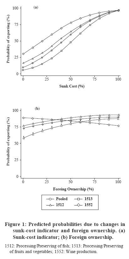
Vegetables; 1552: Wine Production. Based on the above, the predicted probabilities of the export decision arising from the two key firm-specific characteristics: sunk-costs and foreign ownership, were computed. Predicted probabilities due to changes in the sunk-cost indicator (one-period lagged dependent variable) and foreign ownership are presented in Figure 1. For each of these two plots, all other right-hand-side variables were held at their mean. Note the large change in predicted probabilities arising from the sunk-cost indicator (Figure 1a) relative to that of foreign ownership (Figure 1b). These results suggest that larger sunk costs discourage the export decision if firms haven't engaged in export activity, but lead to greater persistence in export activity if firms are already exporters. In other words, a firm that makes investments for exporting in a particular year (sunk costs) will have a higher probability of exporting the next year, because it does not need to incur those costs again. On the other hand, a firm that has not exported in the previous year will have to incur (sunk) costs required for exporting if it wishes to export in the current and future periods. Hence, the presence of sunk costs (export inexperience) will reduce the probability of exporting for domestic market oriented firms. Export intensity Results obtained from the truncated regression model are presented in Table 5. Again, the four specifications correspond to a pooled model and three industry-specific models. Similar to the export-decision results, industry productivity did not have a significant effect on export intensity in any industry. Foreign ownership alone had a positively and statistically significant coefficient only in industries 1513 and 1552 at the 5% and 10% significant level, respectively. As before, foreign investors in these industries may have strong links with their respective home countries (marketing and distribution networks), which likely explains this positive relationship. Size did not show a significant effect in any of the three industries, and highly skilled workers showed a positive and significant effect only in industry 1513. Table 5: Export intensity or level of export production of firms analyzed through a Tobit Model.
1512:
Processing/Preserving of Fish; 1513: Processing/Preserving of Fruits and
Vegetables; 1552: Wine Production. Among the geographical variables, the results are mixed. Infrastructure had a negative and significant effect on the export intensity of industry 1513. This can be explained considering the regional distribution of the infrastructure index (Table 2), and the spatial distribution of export intensity (Region dummy variables of Table 5). The former shows that firms located in the south had a low infrastructure index (except the Magallanes Region), while the latter indicates that firms located in the same zone had higher export production intensity (a positive and significant coefficient of 0.453). Thus, infrastructure and export intensity follow opposite directions. Besides, the construction of the infrastructure index includes industrial capital that was markedly biased in favor of mining capital (Antofagasta Region, a mining region, represents approximately a third of this capital). Thus, an increase of non-agricultural capital will not be related to an increase in the exporter production of the agribusiness and food processing industries. Finally, government quality was positive in industry 1512, but only at the 10% significance level. CONCLUSIONS The export activity of Chilean food processing industries must be analyzed considering the export decision and the export intensity separately. The determinants of exporting behavior vary among sub-industries (four digit ISIC level), and aggregated industrial analyses (two digit ISIC level) could mask the true underlying forces that prevail in each of these sub-industries. The decision to export is strongly influenced by sunk costs. That is, firms that have already exported and invested in the extra costs required for such activities appear to have a higher probability of continuing exporting. Foreign ownership, represented by a percentage of capital stock owned by foreigners, positively impacted on the export decision of the processing/preserving fish industry and the processing/preserving fruits and vegetables industry, a result that has not been reported previously in the literature. Regarding the geographical characteristics, in the agribusiness industry (processing/preserving of fruits and vegetables) infrastructure showed a positive association with the export decision. However, the cumulative effects of geographical characteristics were negative, leaving firm-specific characteristics as the primary determinants of the export decision. Export intensity is also positively influenced by foreign ownership in the processing/preserving of vegetables and fruit and wine production industries. This indicated that foreign investors’ access to marketing and distribution networks likely increases the scale of exports. The effect of geographical variables on export intensity did not show a conclusive result. However, it seems that firms located in the south are expanding their export production faster than firms located in the central zone of the country. In general, firm-specific characteristics significantly impact export behavior in Chilean processed food industries, while the contribution of geography attributes appears mixed. The latter may be due to the use of macro-regional indicators. To better identify geographic effects, micro-level indicators of locational characteristics are needed. Nevertheless, results have provided insights about potential public policies that should encourage participation of the agribusiness and food processed industries in global markets. Given the industry-specific results, further research should focus on analyzing the export decision and intensity at a more disaggregated level. AKNOWLEDGMENTS The authors thank to the Capacity Building Program of The William and Flora Hewlett Foundation and the International Agricultural Trade Research Consortium (IATRC) for supporting this research. Literature Cited
Copyright 2008 - Instituto de Investigaciones Agropecuarias, INIA (Chile). The following images related to this document are available:Photo images[cj08039f1.jpg] [cj08039t2.jpg] [cj08039t1.jpg] [cj08039t4.jpg] [cj08039t5.jpg] [cj08039t3.jpg] | |||||||||||||||||||||||||||||||||||||||||||||||||||||||||||||||||||||||||||||||||||||||||||||||||||||||||||||||||||||||||||||||||||||||||||||||||||||||||||||||||||||||||||||||||||||||||||||||||||||||||||||||||||||||||||||||||||||||||||||||||||||||||||||||||||||||||||||||||||||||||||||||||||||||||||||||||||||||||||||||||||||||||||||||||||||||||||||||||||||||||||||||||||||||||||||||||||||||||||||||||||||||||||||||||||||||||||||||||||||||||||||||||||||||||||||||||||||||||||||||||||||||||||||||||||||||||||||||||||||||||||||||||||||||||||||||||||||||||||||||||||||||||||||||||||||||||||||||||||||||||||||||||||||||||||||||||||||||||||||||||||||||||||||||||||||||||||||||||||||||||||||||||||||||||||||||||||||||||||||||||||||||||||||||||||||||||||||||||||||||||||||||||||||||||||||||||||||||||||||||||||||||||||||||||||||||||||||||||||||||||||||||||||||||||||||||||||||||||||||||||||||||||||||||||||||||||||||||||||||||||||||||||||||||||||||||||||||||||||||||||||||||||||||||||||||||||||||||||||||||
| |||||||||
 [1]
[1]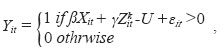 [2]
[2]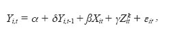 [3]
[3]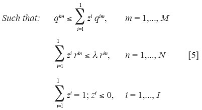