Chilean Journal of Agricultural Research Instituto de Investigaciones Agropecuarias, INIA ISSN: 0718-5820 EISSN: 0718-5839 Vol. 68, Num. 4, 2008, pp. 391-400

Chilean Journal of Agricultural Research (formerly Agricultura Técnica), Vol. 68, No. 4, Oct-Dec, 2008, pp. 391-400

Agricultural labor demand in Chile: a cointegration approach

Demanda por trabajo agrícola en Chile: un enfoque de cointegración.

Rodrigo Saens N.[1]^*, Germán Lobos A.¹, and Edinson Rivera A.[2]

[1]Universidad de Talca, Facultad de Ciencias Empresariales, 2 Norte 685, Casilla 721, Talca, Chile. E-mail rsaens@utalca.cl, globos@utalca.cl * Corresponding author
[2]Research assistant, Universidad de Talca, Chile.

Received: 26 October  2007.
Accepted:17 March 2008.

Code Number: cj08041

ABSTRACT

International evidence shows that the positive relationship between product and agricultural labor has weakened during the last 30 years, especially in emergent economies. Chilean agriculture has not been left out of this phenomenon The main purpose of this reseach was to estimate the causality relationships that govern the product, employment and salaries in the Chilean silviculture-agricultural-livestock sector, using a cointegration approach.Quarterly data from the 1996-2005 period were employed to estimate agricultural labor demand. A Cobb-Douglas agricultural production function was employed and from it were derived the minimum cost function and the labor demand as bases of this study; the latter was approximated log-linearly to find different measures of elasticity. The main results shows that the estimated demand for agricultural labor has long-run employment-product and employment-salary elasticities of 0.38 and -0.88, respectively. An important conclusion suggests that, compared with the employment-product and employment-salary elasticities of labor demand on the aggregated level, agricultural employment in the long run results less sensitive to changes in the product, but more sensitive to changes in salaries.

Key words: agricultural labor, Cobb-Douglas, employment-product elasticity, employment-salary elasticity.

RESUMEN

La evidencia internacional muestra que la relación positiva entre producto y empleo agrícola se ha debilitado en los últimos 30 años, especialmente en economías emergentes. La agricultura en Chile no ha estado al margen de este fenómeno. El objetivo principal de esta investigación fue estimar las relaciones de causalidad que rigen al producto, el empleo y los salarios en el sector silvoagropecuario chileno, utilizando un enfoque de cointegración. Para la estimación de la demanda por trabajo agrícola se utilizaron datos trimestrales del período 1996 a 2005. Se utilizó una función de producción agrícola tipo Cobb-Douglas, a partir de la cual se derivó la función de costo mínimo y la demanda por trabajo base de este estudio; esta última se aproximó log-linealmente para encontrar distintas medidas de elasticidades. Los principales resultados muestran que la demanda por trabajo agrícola estimada presenta elasticidades empleo-producto y empleo-salario de largo plazo de 0,38 y -0,88, respectivamente. Una importante conclusión sugiere que, comparado con las elasticidades empleo-producto y empleo-salario de la demanda por trabajo a nivel agregado, el empleo agrícola en el largo plazo resulta ser menos sensible a cambios en el producto, pero más sensible a cambios en salarios.

Palabras clave: empleo agrícola, Cobb-Douglas, elasticidad empleo-producto, elasticidad empleo-salario.

INTRODUCTION

A central tenet of the neoclassical theory is that labor demand is directly linked to the added product: if the economy grows, so does employment. International evidence shows that the positive relationship between product and agricultural labor has weakened during the last 30 years, especially in emergent economies. According to Klein (1992) and Reardon et al. (2001) during the seventies and eighties, agricultural employment in Latin-american countries fell to almost half; according to Dirven (2004) this fall was intensified in the nineties.

Chilean agriculture has not been left out of this phenomenon As pointed out by Domínguez (2006), the participation of agricultural employment within the total Chilean employment has decreased from 19% in 1990 to 13.8% in 2004. A cursory analysis of the present data indicates that this fall has intensified during the last two years. In December 2006 the average yearly participation of agricultural employment in the total Chilean employment was 12.6% only. Furthermore, agricultural production has increased during 16 years by slightly more than 130%, growing at a yearly rate of 5.4% during the 1990-2006 period, while employment in the sector remained stable at around 800 thousand persons.

Several hypotheses explain what is known in literature as a decline in the employment-product elasticity. According to Weller (2000) the weakening of this relationship would be permanent and structural and its underlying cause would be a technological labor-saving change: the product function would become more capital-intensive over time due to the mechanization of agricultural tasks.

A second hypothesis explaining the weakening of the link between agricultural activities and employment is that this could be occasioned by a temporary reduction in the comparative price of capital versus labor. In effect, according to the results found by Martínez et al (2001), the decrease in employment-product elasticity in the Chilean economy – at the aggregated level, which supposes other constant factors – would not be permanent or structural, but only transitory and could be perfectly well explained by the increases attained by salary during the last years, as compared to the price of capital and other supplies. For example, if the important fall of interest rates experimented by the Chilean economy during the last years is not repeated in future, the growing phase of the cycle would again bring about an increase in the employment-product elasticity, without any modification of the natural unemployment rate of the economy.

There is an important body of literature concerning the Chilean labor market and especially regarding labor demand. For example, Eyzaguirre (1981), Riveros y Arrau (1984) and Paredes y Riveros (1993), estimated a labor demand using data from the manufacturing sector. Marcel (1987), Rojas (1987) and Meller y Labán (1987) performed this exercice using aggregated employment data. However, the results of these studies are quite heterogeneous. One reason could be the scarcity of available data; another, as discussed by Martínez et al. (2001), the absence of cointegration relationships, implying that some of the estimated demands are merely spurious.

This study was a first step to explore the causes underlying the fall experimented by the participation of agricultural employment in the total employment of the economy during the last 16 years.The main objective was to estimate the causal relationships that govern product, employment and salaries in the Chilean silviculture-agricultural-livestock sector. A factor that differentiates the labor market in this sector is the tendency to mechanize agricultural tasks seen during the last two decades, allowing to study the effect of an eventual labor-saving technological change on the Chilean labor market.

MATERIALS AND METHODS

The model

The labor demand is derived from an agricultural production function, which depends on the inclusion of two production factors, capital and labor and is expressed as:

_{y = y (K, L)}                                                                                                                             [1]

where y = agricultural production level, K = amount of capital and L = amount of labor. The reduction of costs problem of each agricultural enterprise is given by the restricted equation:

where c = total production cost expressed in Chilean $; w = cost of labor (salary) expressed in Chilean $ h^-1 and r = opportunity cost of capital expressed in Chilean $ h^-1.

From the first order condition of the restricted minimization problem, can be obtained the labor demand (L^d)  which minimizes the total cost (w, r), conditionned on the product level (y) , is expressed as:

L^d = L^d (w, r, y)                                                                                                                   [3]

If, for example, the agricultural production function were Cobb-Douglas:

y = K^α L^β                                                                                                                                [4]

where α and β are constants  The labor demand would be represented by the expression:

                                                                                                    [5]

Applying natural logarithm to both sides of [5], it is easy to see that for this specific functional form the employment-product elasticity (ε_LY) is represented as: ε_LY = 1/(α+ β). The employment-product elasticity measures the percentage of change in the amount of employment as related to a percentage change in the product level. However, we do not know what is the “true” agricultural production function. What we can observe in practice are the labor hiring and capital factors levels which, in a competitive scenario, minimize the total production cost.

c* = wL* + rK*                                                                                                                     [6]

where L* and K* represent the optimum labor and capital hiring which allow to obtain the minimum cost function, is represented by c*

The Shepard (Nicholson, 1997) precept can be applied to rescue the labor demand function (L^d)  starting from the minimum cost function c*:

                                                                                                [7]

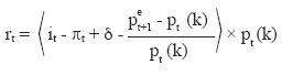
Following Hamermesh (1993) and Martínez et al. (2001), the expression [7] can be approximated log-lineally, to find the labor demand equation, which is the basis of this paper:

log L^d = a₀ + a₁ log y + a₂ log w + a₃ log r                                                                            [8]

where a₁, a₂ and a₃ represent respectively the employment-product, employment-salary and employment-cost of capital of the labor demand elasticities .

The cost of capital for the period t (r_t) is determined by the equation proposed by Romer (2005) and also employed by Bustos et al. (1998) and Martínez et al. (2001):

                                                                                     [9]

where i_t - π_t represents the real interest rate for the period t; that is, according to Fisher’s equation (1930), the difference between the nominal interest rate (i_t)  and the inflation rate (π_t). Coefficient δ is the depreciation rate, p_t (k) is the relative price of capital and  is the capital gain expected by retaining capital during the period t.

Data

The quarterly data from the first quarter of 1990 (1990:1) to the fourth quarter of 2001 (2005:4) period were used to estimate the aggregated labor demand. The employment and salaries series (nominal index of wages deflected by the Consumer Price Index, CPI) were taken from the National Institute of Statistics reports (INE, 2007a; 2007b) and that corresponding to the Gross National Product (GNP) was obtained from Central Bank reports (2007).

For the agricultural labor demand and as the deflector for the silviculture-agricultural-livestock Gross Nacional Product (GNP) was not available for the 1990.1 to 1995.4 period, quarterly data for the period 1996.1 to 2005.4 were used. The series of the silviculture-agricultural-livestock sector GNP were obtained from the Central Bank (2007) and that of agricultural employment from the INE (2007a).  No data after 2006 were used, since in that year the INE introduced changes in the methods employed for the employment survey, making it impossible to set up an adequate overlapping method at this time. 

For the capital cost we considered, as did Martínez et al. (2001), the interest rate reported by the Central Bank for investments for operations at 90 days to one year (basis 360 days) in the financial system deflected by the inflation in 12 months. We also assumed a 10% yearly depreciation rate and as proxy of the price of capital the ratio between the deflector of the gross fixed capital formation and the GNP deflactor, both at the aggregated and the agricultural level. As a way to avoid the unpredictability of the effective capital gains series, the expected capital gains were estimated as the movable average of four quarters in both agricultural and aggregated cases.

When using quarterly data, there can eventually be a relation of dependency between the variable studied and the season of the year in which the measurement was made. Given the nature of the country’s climate, seasonality is especially strong in agricultural economic series. For example, Troncoso y Lobos (2004) found that in the case of fruit and vegetables, the seasonality even influences the wholesale market margins in Santiago, Chile.

In order to obtain a clearer signal of the tendency guiding the levels of employment, product and salaries, seasonality was removed from the series using the Movable Averages Method. Although it is not free from limitations, the technique employed besides being easy, has some features that according to Soto (2002) are desirable in any deseasonalization method: that on applying the method to the deseasonalized series, no new seasonal factors are obtained (characteristic of idem-potency), that the average of the original series should be conserved and that the seasonal components be orthogonal among themselves. No deseasonalization is done using dichotomic variables, since that method assumes that seasonality is a deterministic phenomenon and also, as indicated by Abeysinghe (1994), that the dummies method can induce spurious correlations between the already deseasonalized series.

Unit root test

Two procedures were used to determine the existence of unit roots in each of the series (x_t): (a) the Dickey and Fuller (1984) extended test, and (b) the Phillips and Perron (1988) unit root test. To apply the Dickey and Fuller test, equation [10] includes lags of variable x with the purpose of controlling the autocorrelation serial of the error, that is:

                                                                                [10]

where ε_t is the aleatory term (white noise) which is assumed to follow a normal distribution. To detect the existence of unit root, the null hypothesis H₀: λ= 0 is tested. Zivot and Andrews (1992) and Vogelsang and Perron (1998) show that when the series is not seasonal, the traditional t-Student values for unit roots are not applicable; that is, the significance of the coefficient obtained by means of ordinary means square follow a non standard distribution, so the statistical τ (tau) of Dickey-Fuller must be used.

The Phillips-Perron test, complementary to that of Dickey and Fuller, evaluates the same parameter λ= 0;; however, contrary to the previous procedure, the serial autocorrelation of the error is not controlled by means of lags of x, but by means of the direct correction of the same t-Student statistic.

Cointegration tests

To prove the existente of a long-term relationship between the employment, product, wages and capital cost series, the two-step procedure of Engle and Granger (1987) was used. First a simple linear model is estimated by means of ordinary squared minima and then this is tested to see if the residues of that model are stationary. The cointegration hipótesis was also verifyed using the Likelihood Ratio proposed by Johansen (1988) and Johansen and Juselius (1990). In the first iteration of the Johansen test, the non-existence of a cointegration relationship is the null hipótesis. If this hypothesis is discarded – because the LR is higher than the critical value – the second iteration is evaluated, where the existence of at most one co-integration relationship (against the alternative of more than one) is the null hiypothesis. In the third iteration, the existence of at most two co-integration relationships (against the alternative of more than two) is the null hypothesis. And so successively.

The Johansen cointegration test, based on a generalization of the Dickey-Fuller procedure, determines the number of co-integration equations called “co-integration range”. If there are n co-integration equations, the averages of the series are effectively integrated and the system of autoregressive vectors (VAR) can be reformulated in terms of levels of all the series.

An additional test was used to evaluate the existente of a structural change: the Chow pronostics test (1960) which is used to prove the null hypothesis of the structural stability. That is, if the p value of the F value obtained is low, then the null hypothesis of the structural stability is discarded.

RESULTS AND DISCUSSION

The results of this study show that, considering the increase in the relative cost of the workforce as compared to the cost of capital (w/r) during the 1996 to 2005 period, it is possible to find a stable employment-product relationship during the whole period examined in this research. Therefore, it is possible to disagree with the hypothesis of a structural and permanent fall of the employment-product elacticuty of the agricultural labor demand.

Unit root and cointegration tests

The unit root proofs or tests in the levels and first differences for each of the series are shown in Table 1. The results obtained show that the employment, product, true salary and capital cost series, both on the aggregated as those corresponding to the agricultural sector, are integrated of order one. The results of the Johansen test are shown in Table 2. They show that the existence of a single cointegration vector cannot be discarded; i.e., there is an equilibrium ratio beteen employment, product, salary and capital cost – in the agricultural sector and at the aggregated level – which would allow to estimate a long-term labor demand function. These results are also confirmed by the Dickey-Fuller test (Table 3) which demonstrates the presence of a unit root in the data generation process of the analyzed series. 

Table 1. Presence of unitary roots in the data-generating process: Augmented Dickey Fuller (ADF) and Phillips-Perron tests.

 ¹ At the agricultural level, the critical values, both for the augmented Dickey-Fuller test (ADF) as for Phillips-Perron are: -3.52 and -4.19 for significance levels of 5 and 1% respectively.
² At the aggregated level, the critical values, both for the augmented Dickey-Fuller test (ADF) as for Phillips-Perron are: -3.48 and -4.10 for significance levels of 5 and 1%, respectively.
³ The augmented Dickey-Fuller test is done using a residue, except in the true salary and capital cost of the agricultural sector series, where two residues are used.
Δ: Variation

Table 2. Existence of a single cointegration vector: Johansen cointegration test.

Table 3. Long-run labor demand for labor and demand elasticities for long-run labor

¹ Employment is the dependent variable.
² This was included to reflect the evidence in favor of a structural change in the demand for long and short run agricultural labor during the first quarter of 2001

Long-term labor demand

Table 3 also allows to compare the results of estimating – by ordinary least square – the labor demand of the agricultural sector with its equivalent on the aggregated level. Although the adjustment of the agricultural labor demand model (adjusted R² = 0.72) is lower than that found at the aggregated level (adjusted R² = 0.96), the coefficients are statistically significant in both cases, with signs according to the economic theory and of magnitudes similar to those obtained in Chile by several authors. Among them, the work of Solimano (1981) and Riveros y Arrau (1984) using data of the manufacturing sector, the partial adjustment of the labor demand estimated by Rojas (1987), the aggregated labor demand and another for the manufacturing sector estimated by Paredes and Riveros (1993) and the estimation made by Martínez et al. (2001) used employment data on the aggregated level. The coefficients shown in Table 3 also correspond to the values estimated for long run labor demand elasticities. The employment-product elasticity of the agricultural sector is of 0.38 and of 0.54 on the aggregated level; on the other hand, the employment-agricultural salary elasticity is of -0.88 and at the aggregated level it is of -0.39. Compared to the rest of the economy, long-term agricultural employment shows to be sensitive to changes in the product but significantly more sensitive to changes in salaries.

Structural change in labor demand.

An eventual reason for the weakening experimented by the employment-product relationship of the agricultural sector is a structural change in the labor demand, originating in variables out of the model. For example Martínez et al. (2001) controlling by product level and relative prices, report that Chilean economy demanded less employment at the end of 2000. Likewise, Bergoeing y Morandé (2002) point out that the political discussion of the labor reform taking place at the end of the nineties - which modified the institutional scene governing the labor market, starting on December 1^st, 2001, would have caused a 7% increase of the hiring cost for the Chilean economy as a whole. 

Although the already proven cointegration relationship between employment and its explanatory variables could make the existence of a structural change less probable in principle, an additional test was carried out to prove this change: the Chow forecast test. The results of that test point out the absence of structural change in the aggregated long-term (Table 4) and short-term (Table 5) labor demand. In the case of the agricultural labor demand, however, the Chow forecast test shows evidences in favor of a structural change in the long and short-run labor demand for the first quarter of 2001 (Tables 4 and 5. respectively). The agricultural labor demand in Table 3 includes a dichotomic variable representing that structural change, which proved to be statistically significant, consistent with the first hypothesis of this study.

Table numbers show the p-value.
The dates in the horizontal heading show the cut-off of the estimation sample and the dates in the left column are those for which the test was done. The number after the year refers to the respective quarter.

Table 5. Chow forecast test: short-run labor demand model.

It is also interesting to note that the structural change observed in the agricultural labor demand is not in the employment-product elasticity, but only in the intercept of the function. This structural change could have been occasioned at the time by a single increase in the expected cost of hiring, due, for example, to the uncertainty generated by the discussion of the labor reform implemented at the end of 2001, and/or also, as pointed out by Martínez et al. (2001), to permanent efficiency gains found by farmers affected by the repercussions of the Asian crisis at the end of the nineties. Whatever the case, the present results negates the hypothesis of a secular fall in the employment-product elasticity, either on the aggregated or agricultural level.

Short term labor demand

Although Equation [8] adequately describes the labor demand behavior it is possible that there might be other factors which would cause short runs unbalances. To estimate the adjustment dynamics towards the long-term equilibrium, we employed the error correction method proposed by Sargan (1984) and made known by Engle and Granger (1987). The results of this exercise in Table 6 show that only two variables explain the adjustment of employment towards its equilibrium: the change in the product and the one period lag of the error correction term. In the short-term, agricultural employment or aggregated as may be the case - does not show to be sensitive to changes in salary or to modifications in the cost of capital.

Table 6. Short-run labor demand.

¹Employment is the dependent variable.

As could be expected and in the range of the results found by García (1995) or Martínez(2001), the short-term employment product elasticity - in agriculture as on the aggregated - is smaller than long-term elasticity, shown in Table 3.

CONCLUSIONS:

The analysis of the equilibrium relationships between employment, product and price of production factors for the Chilean silviculture-agricultural-livestock sector allows to reach the following conclusions.

Considering the increase during the last 10 years of the relative cost of the workforce as compared to the cost of capital, it is possible to find an employment-product relationship stable in time, opposing the hypothesis of a structural and permanent fall of this elasticity. Furthermore, this stability is one of the factors allowing to estimate a long-term agricultural labor demand.Sometimes, discussions tend to confuse employment-product arc elasticity with employment-product point elasticity: the first does not condition the result because of change in the relative price of the factors; the second does, as it is a partial derivative of the employment logarithm as respect the product logarythm in a previously estimated demand function.

A statistically significant structural change is observed – of the position, not the slope – in the agricultural labor demand function for the first quarter of 2001.  It is not possible to explain this situation. A likely cause would be the uncertainty generated by the political discussion prior to the labor reform law implemented at the end of 2001; another, the permanent efficiency gains reached by farmers as a consequence of the Asian crisis at the end of the nineties

The values found for the  employment-product and employment-salary elasticities of the agricultural labor demand are 0.38 and -0.88 respectively. Compared with the employment-product and employment-salary elasticities of the labor demand on the aggregated level, agricultural employment in the long run turns to be less sensitive to changes in the product, but more sensitive to changes in the salaries. An explanation could be that the agricultural labour is less qualified, therefore, it can be substituted more easily than that employed in the rest of the economy.

LITERATURE CITED

• Abeysinghe, T. 1994. Forecasting performance of seasonal-dummy models relative to some alternatives. Econ. Letters 44:365-370.
• Banco Central. 2007. Estadísticas económicas. Actividad económica y gasto. Producto Interno Bruto, serie trimestral a precios constantes. Disponible en http://www.bcentral.cl/estadisticas-economicas/series-indicadores/index_aeg.htm (Leído el 17 de abril de 2007).
• Bergoeing, R., y F. Morandé. 2002. Crecimiento, empleo e impuestos al trabajo: Chile 1998-2001. Cuadernos Econ. 39:157-174.
• Bustos, A., E. Engel, y A. Galetovic. 1998. Impuestos y demanda por capital en Chile, 1985-1995. Mimeo. Centro de Economía Aplicada, Departamento de Ingeniería Industrial, Universidad de Chile, Santiago, Chile.
• Chow, G.C. 1960. Tests of equality between sets of coefficients in two linear regressions. Econometrica 28:591-605. 
• Dickey, D.A., and W. Fuller. 1984. Testing for unit roots in seasonal time series. J. Am. Stat. Assoc. 79:355-367.
• Dirven, M. 2004. El empleo rural no agrícola y la diversidad rural en América Latina. Revista de la CEPAL 83:49-69.
• Domínguez, J.I. 2006. Crecimiento, desarrollo y recursos humanos. Agronomía y Forestal 29:6-10.
• Engle, R., and C. Granger. 1987. Cointegration and error-correction: representation, estimation and testing. Econometrica 55:251-276.
• Eyzaguirre, N. 1981. El empleo en una economía deprimida. Análisis econométrico de sus determinantes en la industria chilena 1974-1978. Estud. Econ. 16:45-82.
• Fisher, I. 1930. The theory of interest: as determined by impatience to spend income and opportunity to invest it. 566 p. The Macmillan Co., New York, USA.
• García, P. 1995. Mercado laboral y crecimiento: Chile 1980-1994 y proyecciones de mediano plazo. Colección Estudios CIEPLAN 40:39-70.
• Hamermesh, D. 1993. Labor demand. 444 p. Princeton University Press, Princeton, New Jersey, USA.
• INE. 2007a. Chile estadístico, mercado del trabajo, empleo. Instituto Nacional de Estadísticas (INE), Santiago, Chile. Available at: http://www.ine.cl/canales/chile_estadistico/mercado_del_trabajo/estadisticas_laborales.php (Read April 17,2007).
• INE. 2007b. Chile estadístico, mercado del trabajo, remuneraciones. Instituto Nacional de Estadísticas (INE), Santiago, Chile. Available at: http://www.ine.cl/canales/chile_estadistico/mercado_del_trabajo/estadisticas_laborales.php (Read May 3, 2007).
• Johansen, S. 1988. Statistical analysis of cointegrating vectors. J. Econ. Dynam. Control 12:231-254.
• Johansen, S., and K. Juselius. 1990. Maximun Likelihood estimation and inference on cointegration with applications to the demand for money. Oxford Bull. Econ. Statist. 52:169-120.
• Klein, E. 1992. El empleo rural no agrícola en América Latina. Documento de Trabajo N° 364. 22 p. Programa Regional del Empleo para América Latina y el Caribe (PREALC-OIT), Santiago, Chile.
• Marcel, M. 1987. Empleo agregado en Chile 1974-1985. una aproximación econométrica. Colección Estudios CIEPLAN 21:77-115.
• Martínez, C., G. Morales, y R. Valdés. 2001. Cambios estructurales en la demanda por trabajo en Chile. Economía Chilena 4:5-25.
• Meller, P., y R. Labán. 1987. Aplicación del filtro de Kalman a la estimación  de elasticidades variables en el mercado del trabajo chileno (1974-1985). Análisis Económico 2:41-67.
• Paredes, R., y L.A. Riveros. 1993. El rol de las regulaciones  en el mercado laboral: el caso de Chile. Estud. Econ. 20:41-67.
• Phillips, P.C.B., and P. Perron. 1988. Testing for a unit root in time series regressions. Biometrika 75:335-346.
• Reardon, T., J. Berdegué, and G. Escobar. 2001. Rural nonfarm employment and incomes in Latin America: overview and policy implications. World Devel. 29:395-573.
• Riveros, L., y P. Arrau. 1984. Un análisis empírico de la demanda por trabajo del sector industrial chileno 1974-1982. Estud. Econ. 22:23-46.
• Rojas, P. 1987. Un análisis empírico de la demanda por trabajo en Chile 1977-1985. Cuadernos Econ. 99:251-76.
• Romer, D. 2005. Advanced macroeconomics. 696 p. 3^a ed. McGraw-Hill/Irwin, New York, USA.
• Sargan, J. 1984. Wages and prices in the United Kingdom: a study in econometric methodology. In K. Wallis and D. Hendry (eds.) Quantitative economics and econometric analysis. Basil Blackwell, Oxford, England.
• Solimano, A. 1981. La rebaja en cotizaciones previsionales y su impacto sobre el empleo industrial: una estimación para el período 1974-1978. Notas Técnicas CIEPLAN 48:1-26.
• Soto, R. 2002. Ajuste estacional e integración en variables macroeconómicas. Cuadernos Econ. 39:135-155.
• Troncoso, C., y G. Lobos. 2004. Márgenes de comercialización y concentración industrial en el mercado de frutas y hortalizas en Chile. Agroalimentaria 18:75-86.
• Vogelsang, T., and P. Perron. 1998. Additional tests for a unit root allowing for a break in the trend function at an unknown time. Int. Econ. Rev. 39:1073-1100.
• Weller, J. 2000. Tendencias del empleo en los años noventa en América Latina y el Caribe. Revista de la CEPAL 72:31-51.
• Zivot, E., and D. Andrews. 1992. Further evidence on the great crash, the oil price shock, and the unit root hypothesis. J. Bus. Econ. Statist. 10:251-270.

Copyright 2008 - Instituto de Investigaciones Agropecuarias, INIA (Chile).  

The following images related to this document are available:

Photo images