Chilean Journal of Agricultural Research Instituto de Investigaciones Agropecuarias, INIA ISSN: 0718-5820 EISSN: 0718-5839 Vol. 70, Num. 2, 2010, pp. 315-322

Chilean Journal of Agricultural Research, Vol. 70, No. 2, April-June, 2010, pp. 315-322

Scientific Note

Commercial digital camera to estimate postharvest leaf area index in Vitis vinifera L. cv. cabernet sauvignon on a vertical trellis

Uso de una cámara digital comercial para estimar el índice de área foliar en Vitis vinifera L. cv. Cabernet Sauvignon en poscosecha conducida en espaldera vertical

Espinosa L Miguel¹, Acuña C Eduardo², Espinosa B Miguel², Barrera B Juan³

¹ Viña De Martino, Manuel Rodríguez 229, Isla de Maipo, Chile
² Universidad de Concepción, Facultad de Ciencias Forestales, Victoria 631, Concepción, Chile
³ Universidad de Concepción, Facultad de Agronomía, Av. Vicente Méndez 595, Chillán, Chile

Correspondence Address: Espinosa L Miguel, Viña De Martino, Manuel Rodríguez 229, Isla de Maipo, Chile, mespinosa@demartino.cl

Date of Submission: 06-Jan-2009
Date of Acceptance: 12-Jun-2009

Code Number: cj10034

Abstract

Keywords: Vitis vinifera, leaf area index, digital image, photographic camera

Resumen

En un viñedo (Vitis vinifera L.) cv. Cabernet Sauvignon ubicado en la comuna de Cauquenes, Región del Maule, se estimó el índice de área foliar (LAI) mediante imagen digital obtenida de una cámara fotográfica comercial, a partir de dos métodos indirectos: Espacio y Brillo Área Foliar (LAGB) y Sistema Cuantificador de Área Foliar por Fotogrametría (PLAQS). Este último, requiere el deshoje de la parra. En un mapa de índice vegetativo diferencial normalizado (NDVI), se seleccionaron tres puntos de vigor de las vides: alto, medio y bajo, en cada uno de los cuales se obtuvo una imagen horizontal y vertical. Las imágenes se filtraron con el programa Arc View GIS 3.1, dejando sólo las hojas y el número de píxeles correspondientes. Se calculó el área de la imagen y los metros cuadrados por metro lineal. Se seleccionaron los mejores modelos de tres ajustes de regresión lineal entre: i) el LAI de las imágenes verticales del LAGB con el LAI del PLAQS, ii) el LAI de las imágenes horizontales con el PLAQS, y iii) el LAI de ambos tipos de imágenes con el PLAQS. En todos los modelos los parámetros son significativos. El ajuste entre la imagen vertical del LAGB y el PLAQS, presenta mayor simpleza y facilidad de cálculo, requiriendo sólo una imagen vertical para estimar el LAI. Las imágenes así obtenidas pueden estimar con precisión el LAI en este tipo de cultivar y de conducción de la parra.

Palabras clave: Vitis vinifera, índice de área foliar, imagen digital, cámara fotográfica

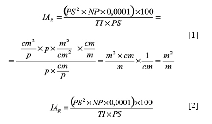
Introduction

The increasing supply of wine products and strong international competition make it necessary to use new technological tools in vineyard management, high quality wines being the final objective. The modernization of vitiviniculture has involved changes in management systems and administration of vineyards to accelerate production, increase yields, and improve grape and wine quality (Lavin et al., 2001).

Cultivar, climate, soil, and production system influence grapevine vigor (Vitis vinifera L.) and its productivity by affecting foliage characteristics regarding the number of shoots per plant, number of leaves per grapevine, and leaf area index.

Appropriate foliage management will improve wine quality, insofar as it influences the microclimate of grape clusters and affects their chemical composition (Mufloz et al., 2002). The quantity and quality of incident light on the plant play an important role. Leaves only absorb part of the light spectrum (especially the visible range), therefore the quantity of light decreases as the light rays go through the foliage affecting fruit color (Bergqvist et al., 2001).

The degree of light that a vineyard requires is a direct function of its leaf surface (Hidalgo, 2006). Leaf surface can increase through crop practices such as irrigation and fertilization thus enhancing the vegetative potential of the plant (Hidalgo, 1999), but possibly producing shade in the vine. The shade affects the must, decreases fruit character in the nose and palate, increases the wine′s herbaceous characteristic, incidence of Botrytis, and prematurely aging the wine (Smart and Robinson, 1991). Bergqvist et al. (2001), Hunter and Archer (2002) point out that one of the main factors that can be affected by canopy development is available radiation for the plant since photosynthetic activity of the leaves along the vine shoot and the transportation of assimilated compounds can increase if they improve foliage microclimatic conditions. So, canopy management techniques are directed towards achieving improvement in the vine light microclimate. In any case, by reducing canopy density to increase radiation, there is also a decrease in negative effects provoked by other microclimate factors influenced by the canopy (Lavin et al., 2001).

Leaf development during the growing season is fundamental to achieve good production in a vineyard due to its importance in intercepting sunlight and for the photosynthesis process (Oliveira and Santos, 1995). Shoot length, pruning intensity, and leaf area index (LAI), among other parameters, are highly important for wine quality (Smart and Robinson, 1991); they are indirect indices appropriate for characterizing the canopy (Dokoozlian and Kliewer, 1995). Therefore, it is necessary to quantify its development to evaluate vineyard vigor during the course of the season and over time (Kusch, 2005).

Plant biomass production is related to light interception which is mainly determined by LAI (Wijk and Williams, 2005). This index depends on the species, state of plant development, and time of year (Jonckheere et al., 2004). Even though it is an important indicator of crop productivity, it is used little in vitivinicultural experiments due to the high cost of direct determination with leaf area integrated electronic equipment (Pire and Valenzuela, 1995) which usually requires destroying the plant (Ollat et al., 1998).

LAI can also be indirectly determined, whether the plant is destroyed or not, with optic devices based on measuring light transmission through the canopy and foliage (Jonckheere et al., 2004). Equipment mostly used to indirectly estimate LAI are the Plant Canopy Analyzer LAI-2000 (PCA Licor, Lincoln, Nebraska, USA) and the Digital Plant Canopy Imager CI-110 (CID Bio-Science, Vancouver, Canada), which both measure transmitted radiation fraction going through the foliage. These instruments are used in a wide variety of agroecosystems ranging from deciduous and coniferous forests to agricultural crops (Johnson and Pierce, 2004; Wijk and Williams, 2005). Another indirect way to determine LAI is with digital images. Digital images are a group of individual elements called pixels which are organized according to a matrix pattern, that is, in rows and columns. Each pixel of the image is subjected to digitalization with the objective of converting the level of light recorded into a numeric value. Therefore, the image is represented as a matrix of numbers, one for each pixel. Digital images maintain the proportions of real objects at any given point in time; their magnitude (length, width, and depth) depends on the focal distance and the distance at which the image was taken, making possible the determination of object size in two or three dimensions (Aristarco, 2009). Digital images are frequently used in the forestry and agricultural areas because of its easy handling, interpretation, and applicable functions (Wulder, 1998).

The objective was to determine the feasibility of using digital images to estimate leaf area in vines by applying two indirect measurement methods: the non-destructive Leaf Area Gap and Brightness (LAGB), and the destructive Photogrammetric Leaf Area Quantification System (PLAQS) using digital photogrammetry.

Materials and Methods

Study Site

The study was carried out in the 2005 postharvest season in the commune of Cauquenes, Maule Region (E 753 401, N 6 013 154, UTM Zone 19S, WGS84) in grapevines cv. Cabernet Sauvignon with photosynthetically active leaves planted on 1.8 m trellises in 1999 with a 3 m space between rows and 1 m over the row. Soils belong to the Cauquenes series (fine, kaolinitic, mesic Typic Palexeralfs), rolling hills with deep low fertility soil. The climate of the area is of subhumid Mediterranean with annual mean rainfall of 695 mm and temperatures fluctuating between 0 and 32ºC (DGAC, 2009).

Determining sampling points

The Normalized Difference Vegetation Index (NDVI) (Rouse et al., 1974) was used as a vegetative expression index map where three levels were selected: high (dark green), medium (light green), and low (yellow) [Figure - 1]. Horizontal and vertical images were obtained in each level to apply the LAGB method and defoliation images for the PLAQS method with three replicates in each sampling point.

Determining leaf area

LAGB Method. This method is based on obtaining light gaps and leaf brightness with horizontal and vertical images. Thus, an Epson (PC500, 2 megapixels, 43 mm lens, Tokyo, Japan) digital camera was connected to a mobile structure at a height of 2.40 m from the ground and 60 cm from the upper surface of the vine [Figure - 2].

A white fiberglass sheet, 6 m ² surface (3 x 2 m) with the longest side parallel to the row, was placed under the vine to obtain horizontal images (top view) [Figure - 3]a. Thereafter, this sheet was located to one side of the vine to obtain a vertical image [Figure - 3]b. Image format was Joint Photographic Experts Group (JPEG) with a 320 x 240 pixel size and transformed into img format to be visualized with ArcView GIS 3.2 software (ESRI, Redlands, California, USA). Leaves were separated from the contrast surface by the activated Image Analysis module of this software. All the pixels containing leaves in the images were selected with Seed Tool resulting in a polygon which is converted from image to shape by the Xtools extension and then shape to grid with the same pixel size as the original image. This grid has two values: 1 and 0; pixels with value 1 are those representing the isolated material and 0 the surface [Figure - 3]c.

The size and total number of pixels of each of the images required to determine leaf surface (square meters per linear meter) was calculated by Equation [1]:

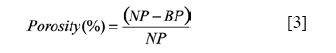
where, IA _R = real image area (m ² m ^-1 ), PS = pixel side (cm), NP = number of image pixels, and TI = horizontal image distance in pixels.

Determining LAGB also allows establishing vine porosity values. In this way, porosity was calculated in each image (ratio of contrast area pixels and vine pixels) by equation [3] (Lamb, 2005):

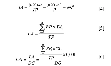
where, Porosity (%) = percentage porosity, NP = number of image pixels, and BP = number of black pixels.

PLAQS Method. Unlike the previous method, this one requires leaf extraction to determine leaf area in the image. Thus, foliage in a linear meter of vine was harvested in each sampling point immediately after taking the image by the LAGB method [Figure - 4]a and put into bags for transport to the laboratory. In the laboratory, leaves were laid out on the 6 m ² white fiberglass sheet [Figure - 4]b and a digital image was taken with an Epson PC500 camera attached to a 2.4 m tripod. The ripple effect of the leaves was not corrected.

Color separation for each image was achieved by Adobe Photoshop 4.0 (Adobe Systems, Seattle, Washington, USA) software. The image was opened in JPEG format, separating the leaves from the contrast surface with the Select Color Range command which allows isolating the areas of an image in accordance with its color channel. A JPEG image contains three color channels with a value spread of 1 to 296 for red, blue, and green. A determined area of an image is selected with this command and all image pixels with identical channel values are simultaneously selected. After color selection, the Edition command changed all the pixels to black (foliage) and white (contrast surface).

Once the image is saved, it is imported by the Idrisi 3.2 software (Clark Labs, Clark University, Massachusetts, USA) defining the reference system (plain), reference units (meters), and distance units (1). To calculate the image, the Image Calculator function was first applied to transform the image to binary and then options of the Area function were selected: output format tabular, input image (upload image to be calculated), and calculate area (as a cell) [Figure - 4]c. Once the number of pixels was obtained, leaf area and LAI were calculated by Equation [6] (Farina, 2006):

where, LAI = leaf area index (m ² m ^-2 ), BP = number of black pixels, TA = total area (cm ² ), TP = total number of pixels, DG = distance between vines (m), ip = image pixels, pa = pattern area (cm ² ), and pp = pattern pixels.

Aberrations were disregarded (e.g. deformation provoked by inclination of the camera optical axis, lack of clarity) in the digital images obtained by the LAGB and PLAQS methods.

Statistical analysis

Linear regression models were adjusted by the Statistix 8.0 software (Analytical Software, 2006): i) LAI of vertical images, measured in m ² m ^-1 , of LAGB method with LAI of PLAQS method, ii) LAI of horizontal images by PLAQS method, and iii) LAI of both types of images (vertical and horizontal) by PLAQS method. The Fumival index (Fumival, 1961), which compares models with distinct dependent variables, was applied to select the best model:

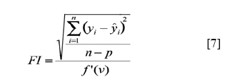
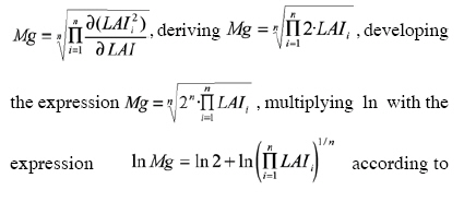
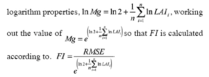
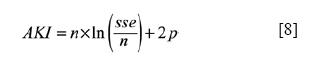
where, FI = Furnival index _yi,= observed values, y _i = estimated values, n = sample size, p = number of model parameters, and f (v) = geometric mean of the first derivative of the dependent variable in relation to LAI.

For example, an equation of the type is equal to LAI² = a + bX³ . Therefore, its dependent variable Y is LAI ² . Then, the geometric mean of the first derivative of the dependent variable in relation to LAI is:

When the models showed distinct parameter numbers, the Akaike index (Akaike, 1974) was applied:

where, AKI = Akaike index, n = sample size, sse = sum square of residuals, and p = number of model parameters.

Results and Discussion

Porosity according to LAGB method, and image area according to LAGB and PLAQS methods [Figure - 5]

shows the variation of the area values of vertical and horizontal images according to sampling points [Table - 1]. Vertical image values are greater in all the sampling points due to the distance at which the vertical image (3.0 m) was taken and also cover a greater leaf surface than the horizontal image (0.6 m).

The methodology adopted estimates LAI and also provides vine porosity values [Figure - 6], inversely proportional to LAGBVER (LAGB vertical). Hidalgo (2006) determined that ideal porosity values fluctuate between 60 and 80%. This study found that 22% of the entries were in this range. The high percentage outside the range (78%) defined by Hidalgo (2006) can be due to bad pruning management, bad fertilization, or deficient application of agrochemicals among other things (Smart et al., 1990; Smart and Robinson, 1991).

Regression model adjustment

The three selected regression models are shown in [Table - 2]. Parameters are significant in all the models, except for e in Equation [10]. Although this equation can show heteroscedasticity of the variance, coefficients continue to be linear and unbiased, but no longer have a minimum variance (Gujarati, 1992). However, this equation achieves greater precision (lower RMSE, FI, and AKI values) though with a greater number of parameters. The values of RMSE and FI are identical in Equations [9] and [10] since the FI denominator is 1, the geometric mean of the first derivative of the dependent variable in relation to LAI, and the numerator is the root mean square error (RMSE) residual. Equation [9] is simpler and easier to calculate since it requires only one vertical image to estimate LAI.

The relationship between LAI from PLAQS and the predictive values of Equation [9] show that all observed values are within the 95% confidence interval [Figure - 6]. Consequently, this equation, which is a function of LAGB, can be used to estimate LAI given the operational and economic advantages of needing only one vertical image.

Destructive methods, such as PLAQS are laborious and require more time than the non-destructive methods (Patakas and Noitsakis, 1999), as well as storage and transportation to the laboratory of the material collected, working I so that FI is calculated unless a portable leaf area meter is available. On the contrary, an indirect and non-destructive method such as LAGB only requires a simple digital camera to estimate LAI. However, software support is needed to calculate the image, a task which can be somewhat arduous. Nevertheless, software can be used for many other purposes along with allowing a large quantity of images to be simultaneously processed and reducing the time to obtain LAI.

The use of digital images taken with conventional photographic cameras, like the one used in this study, has proven to be an appropriate methodology for non--destructive estimates of LAI in different types of crops, agricultural as well as forestry (e.g. Ewing and Horton (1999), Rasmussen et al. (2007) for wheat (Triticum aestivum L.), Blanco and Folegatti (2003) for tomato (Lycopersicon esculentum Mill.), Stewart (2007) for cotton (Gossypium hirsutum L.), and Guevara-Escobar (2005) and Macfarlane et al. (2007) for eucalyptus plantations. Furthermore, as pointed out by Jonckheere et al. (2004), its application is independent of the cloud level and sun inclination degree (zenith angle) on the canopy to obtain a digital image and calculate leaf area since the images are not taken by pointing upwards to the sky.

Conclusions

It is possible to precisely estimate leaf area index in grapevines by an indirect non-destructive method, Leaf Area Gap and Brightness (LAGB). This method uses digital images taken in situ with common digital cameras. It is low-cost, easily implemented, and quickly processed. Furthermore, images can be taken regardless of sky conditions during normal working hours. As for the use of vertical or horizontal images of the LAGB method, vertical images show advantages over horizontal ones since they are simple to calculate and easier to take.

The PLAQS method is also a convenient procedure though more arduous and requiring more time to obtain LAI. However, it can be carried out in both pre- and postharvest with the advantage that the information generated in preharvest can be used for vineyard management.

Future studies should determine the feasibility of the LAGB method in the face of other types of vine management (e.g. double trellis, lire), other cultivars, and vine development stages (e.g. veraison or ripening, preharvest) that would allow discriminating between cluster and leaf, and have implications for vineyard management.^[34]

References

Copyright 2010 - Chilean Journal of Agricultural Research

The following images related to this document are available:

Photo images