Chilean Journal of Agricultural Research Instituto de Investigaciones Agropecuarias, INIA ISSN: 0718-5820 EISSN: 0718-5839 Vol. 70, Num. 3, 2010, pp. 436-445

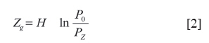
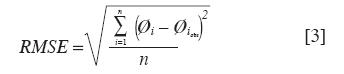
Chilean Journal of Agricultural Research, Vol. 70, No. 3, July-September, 2010, pp. 436-445

Research

Simple air temperature estimation method from Modis satellite images on a regional scale

Método simple de estimación de temperatura del aire a escala regional, a partir de imágenes satelitales MODIS.

P Fabiola Flores, S Mario Lillo

Universidad de Concepción, Facultad de Ingeniería Agrícola, Casilla 537, Chillán, Chile

Correspondence Address: P Fabiola Flores, Universidad de Concepción, Facultad de Ingeniería Agrícola, Casilla 537, Chillán, Chile, fabiolaflores@udec.cl

Date of Submission: 26-Jun-2009
Date of Acceptance: 07-Oct-2009

Code Number: cj10048

Abstract

Keywords: MODIS, atmospheric profile, digital elevation model

Resumen

Para estudios relacionados con la agricultura a escala regional, como balance hídrico y estimación de evapotranspiración entre otros, es importante estimar la variación espacial de la temperatura del aire (Ta), ya que la baja densidad de estaciones meteorológicas no permite obtener dichos datos para una zona determinada. El objetivo de este trabajo fue estimar Ta a partir de perfiles atmosféricos proporcionados por el sensor de imágenes espectroradiométricas de resolución moderada (MODIS) a nivel regional. Una de las metodologías actuales estima la Ta a partir de perfiles verticales de temperatura, por lo que se plantearon modificaciones a dicha metodología en la zonificación, superficie de elevación y relación presión-altitud. Al aplicar esta nueva metodología, las mejores estimaciones de Ta se consiguieron al reemplazar la superficie de elevación del sensor MODIS por la misión topográfica de plataforma radar (SRTM). Finalmente, fue posible estimar la variación espacial de Ta solamente a partir de datos remotamente detectados en zonas de variada geomorfología.

Palabras clave: MODIS, perfil atmosférico, modelo de elevación.

Introduction

Estimating air temperature (T _a ) is very important in monitoring the environment, estimating precipitation, climatic prognoses, determining evapotranspiration, predicting crop yield (Rugege, 2002), and climatic changes (Aikawa et al., 2008) among others. Furthermore, it is the most important meteorological and climatological element, along with radiation, in plant development, determining its spatial distribution, and conditioning agricultural soil suitability (Lozada and Sentelhes, 2008).

T _a is generally measured in meteorological stations by temperature sensors (Unger et al., 2001) located 2 m above the soil surface. The density of these meteorological stations is low (number of station per unit area) to carry out a spatially distributed characterization since there is no data for some large areas (Marquínez et al., 2003). According to Lozada and Sentelhes (2008), one of the main problems in conducting agrometeorological studies is the lack of temperature data. These authors consider that the low density of the meteorological stations in some study areas, addition to flaws in the meteorological data series and/or short historical data series, compromising the quality of estimation of Ta spatially distributed. Most methods to determine T _a spatial variation often use spatial interpolation and extrapolation of data from the nearest meteorological stations. The problem with T _a interpolation and extrapolation is that they depend on many local parameters that can influence its estimation spatially-distributed (e.g. altitude, sun exposure, terrain concavity, and distance from the coast among others) (Marquínez et al., 2003). There are T _a estimation, spatially-distributed, methodologies applied to areas with diverse altitudes using linear interpolation of data provided by meteorological stations (Hernández, 2000; Ibáñez and Rosell, 2001; Cristóbal et al., 2008), as well as those developed for lowlands and valleys where there are no landforms (Unger et al., 2001; Méndez, 2004). This is not the case in Chile, which is located between two mountain ranges, the Coastal Range and the Andes Range. Transverse climatic gradients, from the coast towards the interior, are frequently more emphasized than latitudinal gradients, especially regarding the degree of aridity. A Foehn effect or "rain shadow" is produced behind the coastal elevations, which makes the eastern slopes significantly drier than the western slopes. It is the same for sectors with exposure to the east, which are colder in winter and warmer in summer because they are sheltered from the coastal breeze. This generates sea vegetation gradients toward the interior in almost all latitudes.

The Andes Range acts as a climate zone generator agent with a strong thermal determinant throughout the whole country. Given that temperature decreases about 5 to 6 °C for each 1000 m of altitude, 4000 m mountains can show areas with climatic characteristics with differences of 40 °C over relatively short distances (Santibáñez et al., 2006). To this effect, Price et al. (2000) and Lookingbill and Urban (2003) suggest that the first step in agricultural studies in mountainous regions is the development of simple geographic models to estimate T _a .

The methods actually being used can be divided into two types: those that use information collected on the Earth′s surface and those that employ information obtained through remote sensors (Sánchez and Carvacho, 2006). One of the most used techniques is of the first type and employs a geostatistical algorithm called Kriging with external drift (Hudson and Wackernagel, 1994; Goovaerts, 2000). This is an estimator that incorporates extensively sampled secondary data to characterize the spatial tendency of this variable. In the case of air temperature, Hudson and Wackernagel (1994) introduce terrain elevation as secondary information. The latter significantly improves spatial representation of temperature; however, Kriging with external drift continues to be a variation of a global interpolation method meaning that it depends on the number and distribution of data when interpolating.

T _a can also be estimated from the Earth surface temperature, correlating daily mean air temperature measured in the meteorological stations with surface temperature provided by satellite images. The correlation between diverse air temperatures (maximum or mean, daily or monthly) and surface temperature provided by satellite images is high and allows this variable to be spatially distributed. Errors found in Asturias vary between 1.8 and 2.6 °C (Recondo and Pérez-Morandeira, 2002).

There are also estimation models of environmental variables that incorporate the artificial neural network technique, which acts as a non-linear interpolation tool in tables with multiple entries. Applying these neural networks is a complement for information from scarce data and allows solving the problem of a lack of information in methods such as Kriging. A problem associated with this interpolation process is the discontinuity of climatic conditions, that is, it is difficult to achieve a correct interpolation between such disparate or discrete data (Dolling and Varas, 2002). Geographically Weighted Regression (GWR) models have been developed to explore and describe spatial data, particularly when non-seasonal relationships prevail in space (Brunsdon et al., 1998). Unlike a "normal" linear regression, GWRs assume variations in the spatial relationship parameters (Brunsdon et al., 1999) by carrying out a multiple regression analysis between meteorological and geographic variables to adjust an equation by means of spatial interpolation of data from meteorological stations using tools such as Geographic Information Systems (GIS) and satellite images (Ninyerola et al., 2000; Perry and Hollis 2005, Ninyerola et al., 2007; and Cristóbal et al., 2008). Topoclimatic techniques have also been used to determine spatial distribution of climatic variables through multiple regressions between topographic variables and climatic data showing technological limitations such as the location of the meteorological stations, concentrated in areas less than 1500 m a.s.l. and in the main transverse valleys. Another important aspect is data inconsistency generated by the stations due to technological errors such as failing to update the sensors, their handling, and relocating stations (Morales et al., 2006).

One of the easiest methods to estimate T _a is proposed by Méndez (2004) in the Limpopo River watershed in Mozambique where T _a is estimated from vertical temperature profiles provided by the MODIS sensor. The disadvantage of this method is that it was designed and applied to lowlands or valleys, a condition not always fulfilled in the different zones or regions of Chile.

Lozada and Sentelhes (2008) estimated daily mean temperature (minimum, maximum, and mean) in the Andina Region, Venezuela from a multiple linear regression considering the geographic coordinates (longitude and latitude) as independent variables, and altitude. They based themselves on the fact that the globe′s heat distribution is conditioned by latitude determining availability of solar radiation on the Earth′s surface; by altitude as a product of pressure variation and rarefaction of air; and sometimes by longitude expressing the effect of proximity to the ocean and continentality. The most recent study of T _a estimation is by Esteban et al. (2009) who use the same methodology as the aforementioned authors, but include circulation pattern classification maps in the regression. They incorporate synoptic climatology elements that combine atmospheric circulation with climate and other environmental factors allowing the explanation and forecast of many phenomena and processes taking place in the atmosphere and the environment. According to Esteban et al. (2009), this improves the estimation errors of the variable, but they mention that for a more precise estimate it is necessary to install a network with a larger number of meteorological stations, however, this is too expensive. The problem with this methodology is its local feature since it can only be applied in small sectors due to the fact that there are no circulation pattern classification maps for most countries and spatial distribution of meteorological stations influences in estimation quality.

Most studies to determine T _a are estimates of minimum, maximum, daily, or monthly temperature (Hudson and Wackernagel, 1994; Lookingbill and Urban, 2003; Cristóbal et al., 2008; Esteban et al., 2009), however, determining instantaneous temperature at the time when the satellite passes over the study area is an indispensable element to calculate hydrological variables such as evapotranspiration (Allen et al., 2007) and net radiation (Bisht et al., 2005) on a regional scale. The objective of this study was to estimate T _a (instantaneous) on a regional scale in an area that shows great geomorphological variability using a methodology that only applies data from satellite sensors (remotely sensed) to develop an operational and comprehensive method.

Materials and Methods

Methodology to determine instantaneous T _a from remotely sensed data by atmospheric profiles

The troposphere is the lowest layer of the Earth′s atmosphere and where most meteorological phenomena develop. As altitude from sea level increases, air temperature decreases at a rate of 5 to 6 °C km ^-1 , which is known as adiabatic gradient and Méndez (2004) determined it to be between 1000 and 620 hPa.

In accordance with the above-mentioned, T _a must be determined at an altitude of 2 m above soil surface level according to WMO (2009) recommendations since T _a should be representative of outdoor conditions around the station and also cover an area as large as possible. The methodology proposed by Méndez (2004) to determine T _a is obtained from a linear regression of the vertical temperature profiles (1000 to 620 hPa) and the altitude for each pressure level. The temperature profile was previously determined between observed radiance and the corresponding atmospheric profile by Seemann et al. (2003). Thus, the relationship to estimate T _a at 2 m is Equation [1]:

T_a = m * Z + T₀ [1]

where m is the slope between temperature and elevation, Z is the soil surface elevation plus 2 m, and T ₀ is the temperature at sea level for each pixel. This equation is obtained for each pixel of the satellite image, determining T ₀ at sea level for each pixel.

[Table - 1] shows the different pressure levels with their respective altitudes (WMO, 2009) to implement this methodology independently of the time the satellite passes.

Proposals to improve the methodology to determine instantaneous T _a by remotely sensed data

Taking into account the limitations of the Méndez (2004) methodology to determine T _a , the following modifications were made: Zoning was carried out by separating the study in coastal and central valley areas due to geomorphological variability. Estimated data was compared to the means of the meteorological stations closest to the coast and located at an altitude of less than 150 m. Furthermore, surface elevation provided by MODIS images was substituted by SRTM. This modification was made because the MODIS sensor provides an elevation matrix that differs each day and which can affect the extraction of real data due to some image distortion. Another proposal to improve the determination of T _a was to replace the altitudes for each pressure level provided by WMO for those obtained by Equation [2] (Wallace and Hobbs, 2006):

where Z _g is the surface elevation of the Earth, H = 1/(2.3 FNx01 0.063), P ₀ is the pressure at sea level, 1013.25 hPa, and P _Z is the pressure of Z _g elevation. The authors proposed this modification because the differences between the pressure/altitude ratios [Table - 1] were considerable and directly influenced the determination of T _a .

Satellite images

The study was carried out using images recorded by the MODIS sensor of the Terra (EOS AM) and Aqua (EOS PM) satellites since they provide the temperature profile at different pressure levels and surface elevation necessary to determine T _a . Atmospherically corrected images necessary to implement the methodology were provided by the atmospheric profile MODIS product (MOD07_L2 MODIS) (Wang et al., 2008).

The Terra satellite orbit is regular, going from North to South through the equator in the morning while Aqua goes from South to North over the equator in the afternoon. MODIS provides 36 spectral bands ranging in wavelength from 0.41 to 14.4 μ m; spatial resolution is 250, 500, and 1000 m depending on the product. Another relevant factor when selecting these images is that they are free through the MODIS Website (Xiong et al., 2009).

Surface elevation was provided by SRTM, substituting the one provided by the MODIS sensor for the region under study. SRTM was a mission to obtain a digital elevation model of the area of the globe between 56° lat. S and 60° lat. N in order to generate a complete base of high-resolution digital topographic maps of the Earth. These topographic maps have a spatial resolution of 90 m (Hansen et al., 2009; Houshang and Quiel, 2009) and were georeferenced by the free GlobalMapper (GlobalMapper, 2009) software.

MODIS images were georeferenced by the MODIS Reprojection Tool (MODIS, 2009) program. Image projection corresponded to Mercator Transversal Universal (UTM) with Datum WGS-84 owing to the fact that it is an easy standard system to work with. Digital values provided by MODIS image products were weighted for factors provided by the supplier, obtaining temperature and surface elevation profiles with a spatial resolution of 1 km (MODIS, 2009).

Study area and in-situ data

The study area corresponded to Bío Bío Region, one of Chile′s 15 administrative regions. This region has a wide variability in geomorphology terrain and data availability for comparison and validation. According to the National System of Environmental Information (SINIA), it is the second most important region in terms of population and economic productivity. It covers an area of approximately 37 000 km² ranging from the temperate climate of the central zone with warmer and drier summers which is basically associated with agricultural activities to a wetter climate south of the Laja River where economic activities are mostly related to livestock and forestry. Temperate Mediterranean climatic characteristics predominate in this region with annual precipitation over 1000 mm concentrated between April and November.

Air temperature data measured at the time the satellite passes were provided for 11 meteorological stations distributed throughout the region [Figure - 1] and [Table - 2]. The information is managed by the Instituto de Investigaciones Agropecuarias, INIA Quilamapu located in Chillán, Bío Bío Region, Chile. This network of stations is connected remotely and generates real-time information from different parts of the region.

Stage of analysis

There were two stage of analysis: months with the least cloud cover in the region were considered since cloudiness interferes with data extraction from satellite images; and the range of months studied, October to May, coincided with the irrigation season. The first stage corresponded to the 2005-2006 season, whereas the second considered a more extensive range between 2002 and 2007. Days were randomly selected in each month under study.

Comparison and validation

Air temperature at the time the satellite passes and estimated by the proposed methodology was compared to data from the meteorological stations. Validation of estimated air temperature was performed by comparing the values observed in the meteorological stations and those estimated by the above-mentioned methodology (Equation [3]) through mean squared error (RMSE).

where φ_i and φ_iobs are the estimated and observed values for the i ^th station, respectively, and n is the number of analyzed stations.

The coefficient of determination (R ² ) is the square of the correlation coefficient measuring the intensity of the relationship between two variables, in this case, ambient temperature and surface altitude. R ² measures the degree of dependence between variables and assigns the value 0 for a zero correlation or the value 1 for total correlation.

Results and Discussion

The coefficients of determination (R ² ) between air temperature and surface elevation for all the days of the study and all the analyzed meteorological stations for 273 adjustments varied between 0.98 and 1.

A fairly high RMSE was obtained for some days varying between 1.44 and 7.59 °C. [Figure - 2] shows the relationship between data measured (observed) in the meteorological station located in Chillán and data estimated by the described methodology for the first stage of analysis. The highest RMSE occurred on 10 February 2006. As already mentioned, coastal and central valley areas were divided in order to check if this error was due to the geomorphological condition. Coastal areas raise the value of RMSE on a regional level in the warmest months while these areas show the lowest errors for the coldest months, [Table - 3]. This is attributable to cloud cover in coastal areas on those days and high relative humidity making it difficult to extract data from the image and estimate T _a . The comparison for the coastal areas was based on four meteorological stations located on the coast: Punta Parra, Coronel, Cañete, and Lanalhue, whereas the other seven: El Recreo, Los Maitenes, Coyanco, Portezuelo, Human, Cadepa, and Universidad de Concepción (Chillán) were used to compare the central valley areas.

RMSE was 3.98 °C when 100% of the data was considered as a single set, whereas RMSE was 2.28 °C when 80% of the lower RMSEs were considered, a decrease of 0.72 °C with Sun et al. (2005) who estimated air temperature from the surface temperature in the northern plains of China and obtained a 3 °C error for the best 80% of processed data.

Studies using vertical temperature profiles from the MODIS sensor in the Korean peninsula found errors of 2 °C (Méndez, 2004). These values are acceptable when considering that in the calibration the author used radiosondes with 800 to 400 hPa levels where temperature values are more stable.

According to Menzel et al. (2002), the precision level of the estimates is lower also due to sensor technical factors. The authors reported that sensor input data quality can experience noises and imbalances in the observation angle of the satellite producing 1.9 °C errors in the temperature profiles.

This study was repeated to validate [Table - 3] results by analyzing a series of more comprehensive data in order to verify whether there is a trend or pattern with respect to the zoning carried out, or the warmest and coldest months. Thus, 24 images were considered in this second stage of analysis and general values of RMSE were lower than for the set of previously analyzed days [Table - 4].

There was no pattern or trend because, although RMSE calculated on a regional scale increased in the coastal areas on some days, it was not possible to set a trend as previously thought. Because of this, and bearing in mind that the methodology for determining T _a only uses vertical temperature profiles and surface elevation, geomorphology is not incidental in this methodology.

RMSE was 3.79 °C when considering all the data (100%) in this second stage and decreased in relation to the first analysis while RMSE was 2.64 °C for 80% of the best data, and in this case RMSE was higher than in the previous case though still lower than the 3 °C error obtained by Sun et al. (2005).

Another proposed improvement to the Méndez (2004) model was to substitute surface elevation provided by the MODIS sensor by SRTM. Results generated by including this modification in the application of the methodology to determine T _a are shown in [Table - 4] (SRTM, WMO). In general, RMSE decreased for the different days under study; total RMSE decreased from 3.79 to 3.72 °C, that is, 1.85%. RMSE also decreased from 2.64 to 2.57 °C when considering 80% of the best data, a variation of 2.7%. This decrease was expected since the spatial resolution of surface elevation improved and the same image was used for all the days analyzed.

The last proposal suggested to improve the determination of T _a was to substitute the pressure/altitude ratio provided by WMO (2009) for the one by Wallace and Hobbs (2006) [Table - 1]. Results shown in [Table - 4] (SRTM, W&H) were generated using this variation. RMSE decreased in relation to the original methodology from 3.79 to 3.72 °C (1.85%), however, considering 80% of the best data, it increased 0.4% in relation to the original methodology, that is, from 2.64 to 2.65 °C. The variation of total RMSE was the same as when surface elevation was substituted so that the pressure/altitude ratio proposed by WMO is sufficient to implement this model.

The determination of T _a was also carried out using surface elevation made available by the MODIS sensor and the pressure/altitude ratio provided by Wallace and Hobbs (2006) [Table - 4]. Total RMSE increased 2.6% while the error also increased 3.4% using 80% of the data, fact corroborating that there is no improvement in the determination of T _a by changing the pressure/altitude ratio provided by Méndez (2004) for the one by Wallace and Hobbs (2006).

Green and Hay (2002) compared the results previously obtained with another similar spatial resolution sensor, AVHRR (Advanced Very High Resolution Radiometer) and found a consistent correlation between surface temperature remotely sensed by AVHRR and the monthly T _a observations in meteorological stations in Africa and Europe obtaining a mean RMSE of 4.8 and 3.9 °C, respectively. These errors are higher than those obtained in this study. The difference in actual types of coverage in a 1 km pixel can be misleading when comparing this air temperature data with those monitored by the meteorological station. That is why such errors could decrease when implementing the same methodology with higher spatial resolution images.

[Figure - 3] shows some examples of air temperature maps spatially distributed throughout the region under study acquired by applying the described methodology. Air temperature matches the observed temperature at the time the satellite passes, approximately 15:00 h. The change in shading in these maps can be observed between the coldest and warmest months. It can be observed that temperatures are lower towards the Andes Range area (to the right of each map). Furthermore, temperatures are higher in the central area, which was expected, and a warm temperate climate with a short dry season (less than 4 months) predominates in the central valley areas. [Figure - 4] is an example of results obtained by applying the Kriging interpolation method using only observations from the meteorological stations, and where it can be clearly observed that a higher density of stations is needed to carry out an estimation of T _a spatially distributed.

Conclusions

Study results demonstrated that there is no pattern or trend when zoning is carried out, that is, separating coastal and lowland areas. Furthermore, since the methodology to determine T _a only uses a vertical temperature profile, it is concluded that geomorphology is not incidental in the methodology applied. Nor was there any improvement in the determination of T _a when the pressure/altitude ratio was substituted since altitude decreases in relation to the pressure level and errors increased significantly.

The best air temperature estimate from atmospheric profiles with the proposed modifications was obtained when the MODIS surface elevation was substituted by SRTM attaining errors of 3.72 °C and improving the determination as compared to the original methodology.

Finally, it can be can be concluded that it is possible to estimate air temperature at an altitude of 2 m only from remotely sensed data and that there are differences between real measurements and estimates mainly caused by the heterogeneity of coverage in a 1 km pixel. The hypothesis originated by this methodology in the Bío Bío Region in Chile can be applied in any other region owing to the fact that this proposal is maintained only by using satellite images. It is necessary to emphasize that the methodology to determine T _a applied in this study involves no image and/or software costs.

Acknowledgements

The authors wish to thank the Instituto de Investigación Agropecuarias INIA Quilamapu for providing the data from the meteorological stations distributed throughout the Bío Bío Region, Chile. ^[38]

References

Copyright 2010 - Chilean Journal of Agricultural Research

The following images related to this document are available:

Photo images