Chilean Journal of Agricultural Research Instituto de Investigaciones Agropecuarias, INIA ISSN: 0718-5820 EISSN: 0718-5839 Vol. 70, Num. 4, 2010, pp. 604-615

Chilean Journal of Agricultural Research, Vol. 70, No. 4, 2010, pp. 604-615

RESEARCH

Topoclimatic Modeling of Thermopluviometric Variables for the Bío Bío and La Araucanía Regions, Chile

Elaboración de modelos topoclimáticos de variables termopluviométricas para las Regiones del Bío Bío y La Araucanía, Chile.

Diego Díaz M.^1*, Luis Morales S.², Giorgio Castellaro G.², and Fernando Neira R².

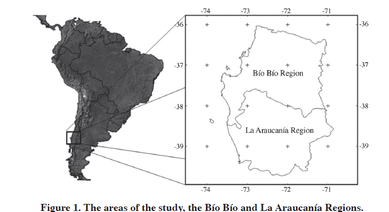
¹Centro Nacional del Medio Ambiente – CENMA, Laboratorio de Modelación e Inventario de Emisiones, Casilla 7880096, Santiago, Chile. ^*Corresponding author (ddiaz@cenma.cl).
²Universidad de Chile, Facultad de Ciencias Agronómicas, Casilla 1004, Santiago, Chile.

Received: 25 August 2009. Accepted: 08 December 2009.

Code Number: cj10068

ABSTRACT

Climatic mapping in the Bío Bío and La Araucanía Regions of Chile is primarily in analog form (paper) and delineation of contours, making it unsuitable for digital handling by geographic information systems (GIS). Therefore, in this study, topoclimatic models were created and spatially represented to explain the spatial and temporal variation of monthly mean temperature and precipitation, as a function of variability and singularity of the physiographic characteristics of the Bío Bío and La Araucanía Regions. The physiographic factors considered were latitude, longitude, altitude, aspect and distance to coastline. To elaborate equations, data from thermopluviometric stations of the study area were compiled and systematized. These stations were standardized to a common reference system in order to locate them in space and obtain the value of physiographic factors for each station. With this information, the equations were calculated using a stepwise (backward) regression procedure, with a statistical significance of 95%. The regression equations obtained for mean monthly and annual temperature and precipitation were all significant (P ≤ 0.05) and had R² > 0.7. These equations were applied to the rest of the study area in raster format using a GIS, which yields a spatially continuous cartography. The spatial resolution or pixel size was 90 m, which allows carrying out research at a 1:100000 scale, commonly used at the regional or provincial level.

Key words: Topoclimatic models, mean temperature, mean precipitation, pluviometric cartographic, GIS.

RESUMEN

La cartografía climática existente en las Regiones del Bío Bío y La Araucanía está fundamentalmente en formato analógico (papel) y con trazado de isolíneas, lo que la hace inadecuada para el manejo digital mediante sistemas de información geográficas (SIG). Por ello, en este estudio se elaboraron y representaron espacialmente modelos topoclimáticos que explicaron la variación espacio-temporal de la temperatura y precipitación en su distribución media mensual, en función de la variabilidad y particularidad de la fisiografía de las regiones del Bío Bío y de La Araucanía. Los factores fisiográficos considerados fueron latitud, longitud, altitud, exposición y distancia a la línea de costa. Para la construcción de las ecuaciones se recopilaron y sistematizaron los datos provenientes de estaciones termopluviométricas de la zona en estudio. Estas estaciones fueron estandarizadas a un mismo sistema de referencia, con la finalidad de localizarlas en el espacio y obtener los valores de sus factores fisiográficos. Con esta información se calcularon las ecuaciones mediante un procedimiento de regresión “stepwise”en su forma “backward”, con una significancia estadística del 95%. Las ecuaciones de regresión obtenidas para las temperaturas y precipitaciones medias mensuales estudiadas fueron significativas (P ≤ 0,05) y con coeficientes de determinación que superaron 0,7. Estas ecuaciones fueron representadas espacialmente utilizando SIG de tipo raster. La resolución espacial o tamaño de píxel empleado fue de 90 m, la que permite realizar estudios a una escala aproximada de 1:100000, que es comúnmente utilizada en análisis de carácter regional y/o provincial.

Palabras clave: modelos topoclimáticos, temperaturas medias, precipitaciones medias, cartografía termopluviométrica, SIG.

INTRODUCTION

Climate, defined as the mean state of the atmosphere in a determined place, is a variable that affects, models and conditions biological, physical and chemical processes that occur in nature (Hufty, 1984). The elements influenced by climate are geography, soil characteristics, vegetation, and ultimately the use and occupation of a determined territory. Because of this, the climatic variable is a conditioning factor in the planning of human activities (Romero and Martínez, 2001). If we consider the importance of climate for the processes that occur in nature and the possible variations of climate owing to physiographic factors, it is necessary to have base climatic information to undertake any study about a determined territory.

This is relevant for Chile, where the physiographic factors are highly variable, with a latitudinal range of approximately 38º (Di Castri and Hajek, 1976), altitudes that range from 0 to 6000 m.a.s.l. and a marked maritime influence (Errázuriz et al., 1994). The study of climatic variation attributable to physiographic factors has been undertaken using what is termed “topoclimatic analysis”, which is defined in general terms as the climatic characteristics of a place that can be described as a combination of topographic parameters (Okolowicz, 1969, cited by Kaminski and Radosz, 2005). The cartographic representation of climatic variables has generally been carried out manually, subject to expert criteria, such as isothermal and isohyet maps, which are isolines that join points with the same temperature and the same level of precipitation, respectively. These isolines are drawn on the basis of an altitudinal gradient, considering the values registered each year from observatories in the zone, the density of which conditions the interval of its plotting (Fernández, 1996). As an alternative to this method of representation, different interpolation algorithms have been developed and automated to estimate and predict the spatial distribution of a variable based on timely data generated by meteorological stations (Hijmans et al., 2005; Hunter and Meentemeyer, 2005; Attorre et al., 2007).

The processes of obtaining climatic cartography, whether through the use of a traditional methods (analogic) or an automated method, is conditioned by the availability and quality of climatic information or data that comes mainly from meteorological stations located in particular points in space (Skirvin et al., 2003; Morales et al., 2006) that often do not cover the totality of a region, leaving areas without information. Given this, models are developed that allow for spatially representing the monthly distribution of temperature and precipitation on an ongoing basis, using Geographic Information System (GIS) raster, obtaining Digital Terrain Models (DTM), which are spatial representations of continuous variables (Doyle, 1978; cited by Florinsky, 1998; Daly et al., 2008). Given the importance of having climatic information to develop studies in a determined area, and considering the physiographic variability of Chile associated with the lack of good coverage by meteorological stations and the continuous character of the distribution of climatic variables, this study aims to generate estimation models of climatic information that allow for continuously characterizing the whole territory, taking into consideration physiographic variables.

MATERIALS AND METHODS

Area of study

The study was carried out in the Bío Bío and La Araucanía Regions, central Chile (36°0’ to 39°38’ S; 70°49’ to 73°57’ W) covering an approximate surface area of 68 704 km² (Figure 1 ). The Bío Bío Region marks a transition from the temperate climate that characterizes the central zone of Chile and the rainier climate characteristic of areas south of the Laja River. The characteristics of a temperate Mediterranean climate predominate in this region. Nevertheless, differences are observed within the territory, fundamentally owing to the effect of the latitudinal gradient and the distance from the coast. The La Araucanía Region presents two well-differentiated climatic typologies, the first located in the intermediate zone in the north of the region until around 39º S lat, characterized by precipitation distributed throughout the year and a relatively short dry season of no more than 3 or 4 months during the summer. The second zone is characterized by a temperate rainy climate with Mediterranean influence, while extends until Castro in the Los Lagos Region.

Climatic and topographic data

Data was used for this research from stations with ten or more years history of taking climatic measurements (Table 1) derived from: Climatology in Chile (United Nations Development Program UNDP - Government of Chile, 1964), Agroclimatic Map of Chile (INIA, 1989), General Water Directorate (DGA) and yearbooks from the Meteorological Directorate of Chile (DMC). To spatially represent the equations, four Digital Terrain Models were used, with information on latitude, longitude, exposure and distance from the coast, and a Digital Elevation Model obtained from the Shuttle Radar Topography Mission (SRTM), of the United States Geological Survey (USGS, 2004), all of them with a pixel size of 90 m.

Table 1. Meteorological stations used in the temperature models.

NE: not specific (INIA, 1989).

To adjust the temperature model, only the stations that had data for more than 10 yr were considered, from the four aforementioned sources. On the other hand, owing to the greater spatial and temporal variability of precipitation, only data from DGA stations with ten or more years of sampling records were used (Table 2). For the development, adjustment and spatial representation of topoclimatic models, it is necessary to homogenize the information, given that the stations that provide information have different reference systems, so that all the information of a geographic character was worked in the World Geodetic System (WGS84) in spherical coordinates. Subsequently, the database was completed that was used for the generation and spatial representation of the topoclimatic models. The physiographic variables included in this study were altitude, latitude, longitude and distance from the coast. All these variables were represented with a pixel resolution of 90 m, which was used for the spatial representation of topoclimatic models and is responsible for the continuous character of the cartographies of temperature and precipitation that were generated. Once the equations have been estimated, thematic cartographies of a continuous character were developed using the computer program IDRISI^® (IDRISI 32, Clark Labs, Clark University, Massachusetts, USA) and the MDTs of latitude, longitude, altitude and distance to the coast.

Table 2. Meteorological stations used in the precipitation models

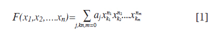
Topoclimatic modeling

The modeling of different climatic variables was done by applying a mathematical model described by Equation [1]:

where F(x₁, x₂ ,.....x_n) represents a climatological variable in a given period of time, x is a descriptor variable, which can be latitude, longitude, altitude, distance from the coast or slope, among others, and a_j are coefficients to be determined (Qiyao et al., 1991; Canessa, 2006). With these relationships, the data matrices are calculated for each climatological variable in binary format (raster) for the months of January and July. The binary metrical format was used because it corresponds to the format of the IDRISI Program^®, which is used for the spatial characterization of continuous variables. The proposed topoclimatic model (Equation [1]) to estimate mean monthly temperature and precipitation considered that spatial variation of the aforementioned variables is determined by factors of position on the surface of the earth, this being latitude (LAT, degrees) and longitude (LON, degrees), as well as physiographic factors like altitude (ALT, m.a.s.l.) and distance to the coast (DL, km), as shown in Equation [2].

Y = a₀ + a_lLAT + a₂LON + a₃ALT + a₄DL [2]

where Y represents mean monthly temperature and precipitation estimated for each month, while the values a₀, a₁…a₄ are coefficients of the corresponding equation. All the models represented by Equation [2] were submitted to a stepwise regression procedure in its backward form, with the aim of finding the reduced models of greater statistical significance. The goodness of fit of all the topoclimatic regressions previously described was calculated with a statistical significance of 95% (P ≤ 0.05), both for the complete model and for each one of its coefficients. To validate the models, four stations were used for the case of temperature (Table 3) and eight for precipitation (Table 4). The spatial coverage of the available stations was analyzed to choose the stations for validation, selecting those that were distributed all along the zone under study, avoiding stations that were isolated from other stations. As well, to minimize errors in the administrative boundaries of the two regions, stations outside the area of study were considered.

Table 3. Selected stations for the validation of the models of mean monthly temperature

Table 4. Selected stations for the validation of the models of mean monthly precipitation

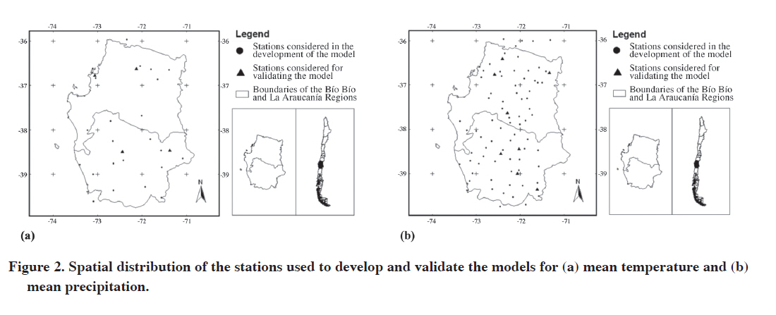
RESULTS AND DISCUSSION

To calculate the models, 25 stations with temperature information and 74 stations with precipitation information were used, which meet the requirement of ten or more years of records. The spatial location of the selected stations is presented in Figures 2a and 2b.

The distribution of stations with temperature data has a low density and representativeness in the Bío Bío Region (Figure 2). As well, it can be observed that the stations with pluviometric data are mainly concentrated in the intermediate valley of the area of study, without information from the coastal Nahuelbuta mountain range or areas above 1200 m.a.s.l. in the Andean Range. Given this, the authors recommend not including aforementioned zones for the estimation of the models.

Estimation of mean monthly temperature (TMMest_(i), ºC)

To estimate TMMest_(i) (where i corresponds to the months of the year), the general model of Equation [1] was used and the values corresponding to coefficients a_n were obtained with the backward stepwise analysis (Table 5). The models generated for the different months were significant to a level of confidence of 95% (P ≤ 0.05), explaining over 60% of the variation of the data and the standard error was less than 1.5 ºC. The descriptor variable used resulted significant with 95% of confidence.

Table 5. Values of the regression coefficient that notes the dependence of mean monthly temperature (TMMest) on physiographic variables according to Equation [2].

With these values, the mean monthly temperatures of the stations selected for validation of the models (Table 6).

Table 6. Statistical summary of the stations with mean monthly temperature considered for the validation

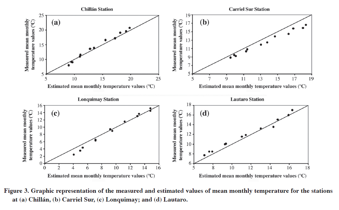
The statistical difference between what was measured and what was estimated for the four seasons indicate that the regressions are all significant to 95% of confidence (P ≤ 0.05, Table 6). The determination coefficients indicate that the models explain over 98% of the variation observed in the data and the standard error was lower than 0.5 ºC. These results are presented graphically in Figure 3.

An overestimation of the model can be observed in Figure 3b. This could be explained by the proximity of the Carriel Sur station to the Concepción station, the latter being within the city, while the former is located some 8 km from Concepción. Concepción has higher mean temperatures owing to the “caloric island” effect associated with populated centers (Rivero, 1988 cited by Navarrete et al., 2001).

Estimation of mean monthly precipitation (PPMest_(i), mm)

As was done for the mean temperature models, the general model of Equation [2] was used, and the values corresponding to coefficients a_n were obtained with backward stepwise analysis. The models generated for different months were significant to a level of confidence of 95% (P ≤ 0.05, Table 7), explaining over 60% of the variation in the data and the standard error was less than 70 mm. The descriptor variables used resulted significant with 95% of confidence.

Table 7. Values of the regression coefficient that notes the dependence of mean monthly precipitation (PPMest) on physiographic variables according to [2].

Mean monthly precipitation was estimated with these values from the stations selected for validation of the models. The regression statistics for the validation stations are presented in Table 8.

Table 8. Statistical summary of the stations, with monthly mean precipitation data considered for the validation.

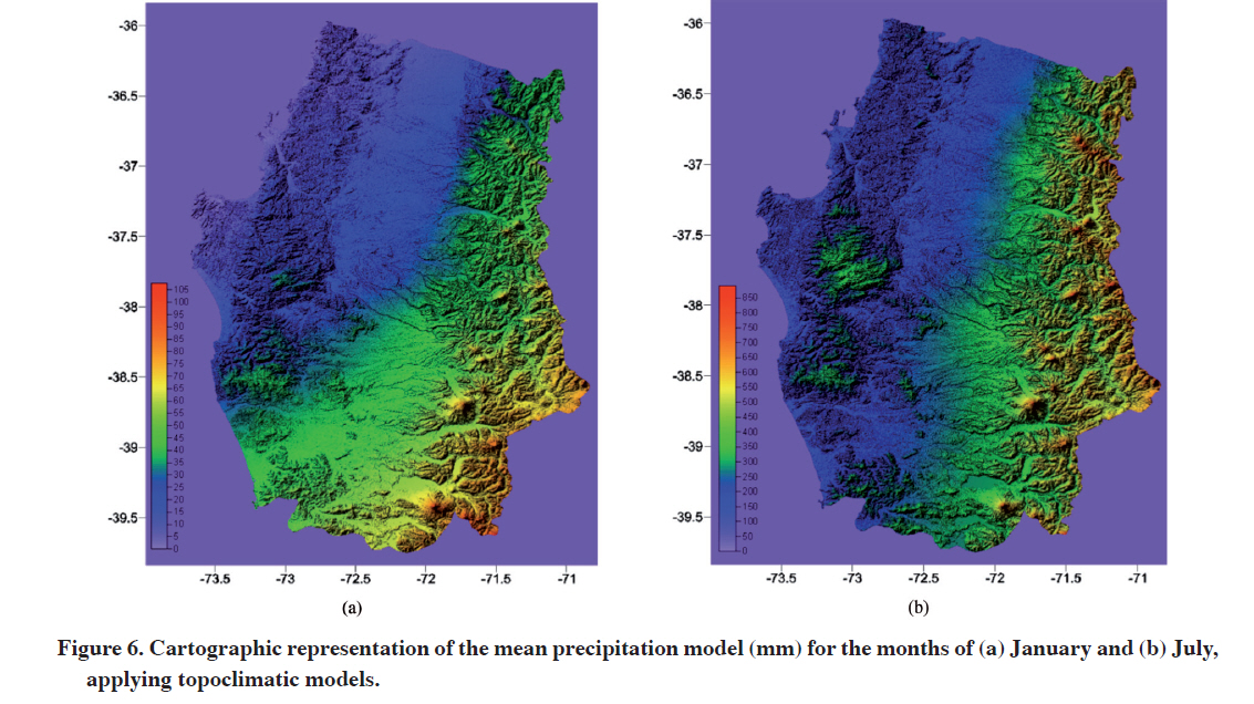
The statistical difference between what was measured and what was estimated for the eight stations of validation indicate that the regressions are all significant to 95% of confidence (P ≤ 0.05). The determination coefficients indicate that the models explain over 92% of the variation observed in the data and the standard error was less than 32 mm (Table 8). The graphic representation of the models for the eight seasons is presented in Figure 4.

The calculated models show significant statistical values (P ≤ 0.05), and the values of R² in the majority of the estimations are higher than 70%. These values are within the range of those obtained in other studies of a topoclimatic character undertaken in Europe by Ninyerola et al. (2000), who reports values of R² higher than 70% for the estimation of precipitation and higher than 86% temperature. In turn, the studies of Goodale et al. (1998) indicate values higher than 69% for the estimation of mean precipitation. Nevertheless, these studies have a high density of stations, greater than those used in this work. As well, the regions where the models are developed tend to present less geographic complexity than is found in the zone under study.

Spatial analysis with thermopluviometric data is problematic because meteorological stations that operate under different institutions provide information using distinct cartographic reference systems that rarely have detailed databases. As well, the stations lack strict spatial location, considering only a level of exactitude of degrees and minutes of longitude and latitude. To resolve this problem there should be a homogenization and documentation criterion of the location of meteorological stations in space in a unique reference system and incorporate exactitude to the level of latitudinal/longitudinal seconds.

A continuous model of climatic variables facilitates carrying out environmental studies of a local character, allowing for deriving a range of models that have the thermopluviometric characteristics of a determined place as independent variables.

This work is a starting point to improve models of a topoclimatic character, whether by the quality and quantity of stations with thermopluviometric data or by the incorporation of new factors that modify the space-time variability of precipitation and temperature. Among the factors that could be included to improve the models is the use of satellite images, specifically spectral indices, reflectivity and surface temperature (Pesquer et al., 2007). For other meteorological variables, such as extreme mean monthly temperatures, we believe that it is possible to apply the same method.

Spatial representation of the models

Figure 5 and 6 show the cartographic results of the application of temperature and precipitation models.

CONCLUSIONS

It was possible to estimate the spatial distribution of the mean values of precipitation and temperature with statistical reliability of 95%, through the generation of topoclimatic models based on multiple linear regressions with descriptor variables, such as position (latitude, longitude, altitude and distance to the coast).

Despite the extreme physiographic variability of the territory under study and the low density of meteorological stations, the topoclimatic models satisfactorily estimated mean monthly and annual temperature and precipitation in vast areas lacking stations, such as the Nahuelbuta Range.

The method developed allows for storing the results in binary matrices compatible with geographic information systems, which in turn allows for calculating other derived variables, such degree-days and chilling hours, which are very useful for studies of agricultural adaptability.

AKNOWLEDGEMENTS

Thanks to the General Water Directorate for facilitating access to a major part of the meteorological data used in carrying out this study.

LITERATURE CITED

1. Attorre, F., M. Alfo, M. De Sanctis, F. Francesconia, and F. Brunoa. 2007. Comparison of interpolation methods for mapping climatic and bioclimatic variables at regional scale. International Journal of Climatology 27:1825-1843.
2. Canessa, F. 2006. Evaluación de los recursos climáticos de la IV Región de Coquimbo, mediante la utilización de Topoclimatología e imágenes NOAA-AVHRR. Tesis Ingeniería. Universidad de Chile, Facultad de Ciencias Agronómicas, Santiago, Chile.
3. Daly, C., M. Halbleib, J. Smith, W. Gibson, M. Doggett, G. Taylor, et al. 2008. Physiographically sensitive mapping of climatological temperature and precipitation across the conterminous United States. International Journal of Climatology 28:2031-2064.
4. Di Castri, F., y E. Hajek. 1976. Bioclimatología de Chile. 129 p. Editorial Universidad Católica de Chile, Santiago, Chile.
5. Errázuriz, A., P. Cereceda, J. González, M. González, M. Henríquez, y R. Rioseco. 1994. Manual de geografía de Chile. 415 p. Editorial Andrés Bello, Santiago, Chile.
6. Fernández, F. 1996. Manual de climatología aplicada. Clima, medio ambiente y planificación. 285 p. Editorial Síntesis, Madrid, España.
7. Florinsky, I. 1998. Combined analysis of digital terrain models and remotely sensed data in landscape investigations. Progress in Physical Geography 22:33-60.
8. Goodale, C., J. Aber, and S. Ollinger. 1998. Mapping monthly precipitation, temperature and solar radiation for Ireland with polynomial regression and digital elevation model. Climate Research 10:35-49. Available at http://www.int-res.com/articles/cr/10/c010p035.pdf (accessed 26 November 2005).
9. Hijmans, R., S. Cameron, J. Parra, P. Jones, and A. Jarvis. 2005. Very high resolution interpolated climate surfaces for global land areas. International Journal of Climatology 25:1965-1978.
10. Hufty, A. 1984. Introducción a la climatología. 292 p. Editorial Ariel, Barcelona, España.
11. Hunter, R., and R. Meentemeyer. 2005. Climatologically aided mapping of daily precipitation and temperature. Journal of Applied Meteorology 44:1501-1510.
12. INIA. 1989. Mapa agroclimático de Chile. 221 p. In Novoa, R., y S. Villaseca (eds.) Instituto de Investigaciones Agropecuarias INIA, Centro Regional de Investigación La Platina, Santiago, Chile.
13. Kaminski, A., and J. Radosz. 2005. Topoclimatic mapping on 1:50000 scale, the map sheet of Bytom. Available at http://www.geo.uni.lodz.pl/~icuc5/text/P_8_1.pdf (accessed 18 May 2005).
14. Morales, L., F. Canessa, C. Mattar, R. Orrego, y F. Matus. 2006. Caracterización y zonificación edáfica y climática de la Región de Coquimbo, Chile. Revista de la Ciencia del Suelo y Nutrición Vegetal 6(3):52-74.
15. Navarrete, G., J. Hernández González, A. Capelli De Steffens, y M.C. Píccolo. 2001. La isla de calor estival en Temuco, Chile. Papeles de Geografía 33:49-60.
16. Ninyerola, M., X. Pons, and J. Roure. 2000. Climatological modeling. A methodological approach of climatological modeling of temperature and precipitation through GIS techniques. International Journal of Climatology 20:1823-1841.
17. Pesquer, L., J. Masó, y X. Pons. 2007. Integración SIG de regresión multivariante, interpolación de residuos y validación para la generación de rásters continuos de variables meteorológicas. Revista de Teledetección 28:69-76.
18. Programa de las Naciones Unidas para el Desarrollo (PNUD)-Gobierno de Chile. 1964. Proyecto Hidrometeorológico. Climatología en Chile. Fascículo I. Valores normales de 36 estaciones seleccionadas. Período 1916-1945. s.e. Santiago de Chile. s.p.
19. Qiyao, L., Y. Jingming, and F. Baopu. 1991. A method of agrotopoclimatic division and its practice in China. International Journal of Climatology 11:86-96.
20. Romero, R., et J. Martínez. 2001. La cartographie climatique dans la planification des zones de protection spéciale d'oiseaux. In XIV Congreso Internacional de Climatología, Sevilla, España. 12-15 septiembre 2001. Association Internationale de Climatologie & Universidad de Sevilla. Available at http://www.juntadeandalucia.es/medioambiente/clima_atmosfera/posters1.pdf (accessed 14 July 2005).
21. Skirvin, S., S. Marsh, M. McClaranw, and D. Mekoz. 2003. Climate spatial variability and data resolution in a semi-arid watershed, south-eastern Arizona. Journal of Arid Environments 54:667-686.
22. USGS. 2004. Shuttle radar topography mission, 3 Arc Second scene. Unfilled Unfinished 2.0. Global Land Cover Facility. Febrero 2000. University of Maryland, College Park, Maryland, USA.

Copyright 2010 - Chilean Journal of Agricultural Research

The following images related to this document are available:

Photo images