 |
| About Bioline | All Journals | Testimonials | Membership | News |
|
||||||
|
||||||
Chilean Journal of Agricultural Research, Vol. 71, No. 2, April-June, 2011, pp. 175-186 Research Genotype × Environment Interaction in Canola (Brassica napus L.) Seed Yield in Chile Interacción genotipo × ambiente en el rendimiento de semilla de raps (Brassica napus L.) en Chile. Magaly Escobar1*, Marisol Berti1, Iván Matus1, Maritza Tapia1, and Burton Johnson2 1 Universidad de Concepción, Facultad de Agronomía, Av. Vicente
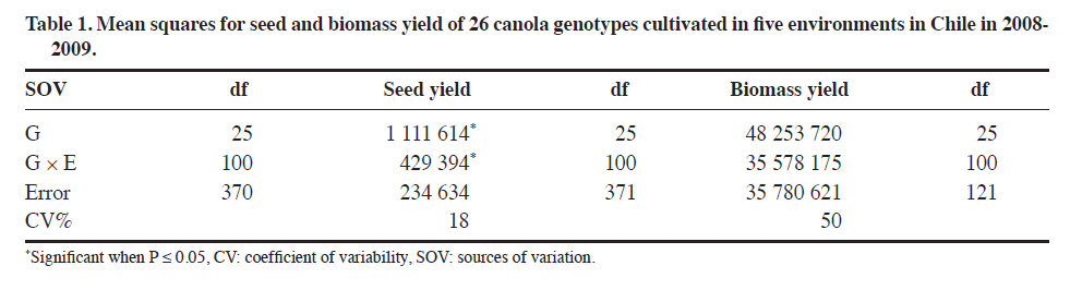
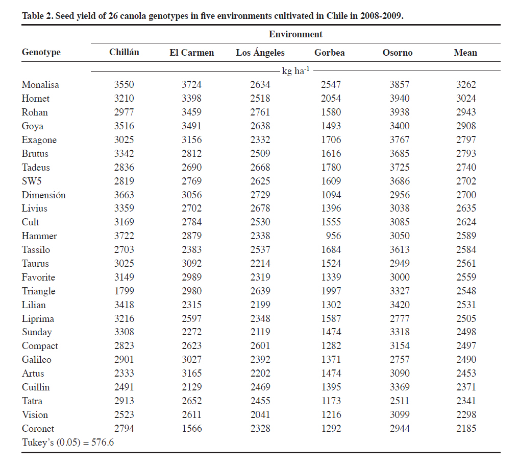
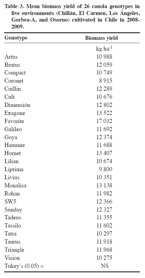
Méndez 595, Chillán, Chile. Received: 25 March 2010. Code Number: cj11021 ABSTRACT Genotype x environment (G × E) interaction in canola (Brassica napus L.) cultivar seed yield is unknown in Chile. The interaction was performed with the SREG (Sites Regression) model. Two experiments were conducted in five and thirteen environments in the 2008-2009 season in Central South Chile. The experimental design was a randomized complete block (RCBD) in each environment with four replicates and 26 open-pollinated or hybrid canola genotypes in Experiment 1, and RCBD with three replicates and 17 genotypes in Experiment 2. ANOVA was used to determine the significance of the G × E interaction. Biplots were used to graphically interpret and determine the best cultivar in each environment and the corresponding mega-environments. The G × E interaction was significant for seed yield in many locations in one cropping season. Most of the analyzed seed yield variation was due to environment and G × E effects. Principal components (PC1 and PC2) of the Sites Regression (SREG) model, with five and eight environments, accumulated 74.5% and 61.1% of the total variation, respectively. Two mega-environments were formed; the first being the Chillán environment while the second included the remaining environments. Six of the evaluated cultivars, all hybrids except ‘Goya’, were superior. The mean vs. stability analysis indicated that the Monalisa hybrid had the highest yield and was the most stable cultivar across all environments. Although the information is for only 1 yr, results could change with data from several years of experimentation. Hence, the study was carried out in many locations in order to provide validity to the results. Key words: SREG, GGE, MET, interaction, biomass, Brassica napus. RESUMEN La interacción genotipo x ambiente en raps (Brassica napus L.) en Chile es desconocida. Para su determinación se utilizó el modelo SREG (regresión de sitios). Dos experimentos fueron establecidos en la temporada 20082009. El diseño experimental en cada ambiente fue de bloques completos al azar con cuatro repeticiones y 26 cultivares de polinización abierta o híbridos de raps para el Experimento 1 y de bloques completos al azar con tres repeticiones y 17 cultivares para el Experimento 2. Se utilizó un ANDEVA para determinar la significancia de G × E. Se usó el biplot para la interpretación gráfica y determinación del cultivar superior en cada ambiente y determinar el correspondiente mega ambiente. En una temporada y para las localidades evaluadas la interacción G x E fue significativa para rendimiento de semilla. La variación en el rendimiento de semillas determinada por el análisis fue debido al efecto del ambiente y de la interacción G x E. Los componentes principales (PC1 y PC2) del modelo SREG con cinco y trece ambientes acumularon 74,5% y 61,1% del total de la variación, respectivamente. Se formaron dos mega ambientes, un ambiente representado por Chillán y el otro formado por el resto de los ambientes estudiados. Seis de los cultivares evaluados fueron superiores y todos fueron híbridos excepto ‘Goya’. El análisis del promedio vs. estabilidad indicó que el híbrido Monalisa fue el de mayor rendimiento y el más estable evaluado a través de todos los ambientes. La información presentada sólo representa una temporada y podría variar si incluyera información que cubriera algunos años. Palabras clave: SREG, GGE, MET, interacción, biomasa, Brassica napus. Worldwide canola production is approximately 50 million tons and covers a total area of 27 million hectares. The main producers are China, 49%; the Economic European Community, 25%; Canada, 12%; and India, 9% (FAOSTAT, 2010). The total area of canola in Chile in the 2008-2009 season was 25 135 ha which produced oil and meal for the bovine and fish food industries (ODEPA, 2009). The environment is the sum of all external conditions affecting cultivar growth and development. Soil texture, pH, depth, organic matter, fertility, diseases, and insects contribute additional variability to the environment (Roozeboom et al., 2008). The genotype × environment interaction (G × E) is the response of each cultivar to variations in the environment (Crossa et al., 1991). The G × E interaction has been one of the principal subjects of study in breeding, allowing the generation of different methodologies for genetic improvement. It has also been a constant worry for breeders, especially when the magnitude of G × E is large, since this impedes the selection and recommendation of stable cultivars, as well as slowing selection advancement (Rodríguez et al., 2002). In many countries, before a cultivar is released for production, government authorities usually require at least 3 yr of performance tests in different environments. There are two possibilities to develop cultivars with low G × E interaction: subdivide areas in relatively homogeneous regions where cultivars need specific adjustment, or generate high stability materials adapted to a wide range of environments. The ideal cultivar would be the one with high seed yield and high stability when evaluated across different environments (Yan et al., 2007). Multi-environment trials must be established mainly to identify the best cultivars for a location and then determine if locations can be established as mega-environments (Yan et al., 2000). Zobel et al. (1988) compared traditional statistical analyses such as ANOVA, Principal Components Analysis (PCA), and linear regression to demonstrate that they were not always effective in analyzing test information in multiple environments. ANOVA is an additive model that describes principal effects and determines if the G × E interaction is significant, but it does not discuss in depth the reasons for this. Principal Components Analysis is a multiplicative model that does not contain the origin of the variation for the principal additive effect of the cultivar or the environment, and does not precisely analyze the interaction. The linear regression method uses the environment means for which estimates are frequently weak or poor and gives information about a small fraction of the total variation generated by the G × E interaction. The biplot is a useful tool to visually evaluate and interpret cultivar response patterns, environments, and the G × E interaction. The biplot is a graphical representation of the simultaneous behavior of two variables. Biplots were originally proposed by Gabriel(1971) and are useful to analyze and summarize a great quantity of information through graphing (Crossa et al., 1991; Gauch, 2006). The biplot is also used to interpret analysis results of the Sites Regression (SREG) model of the information obtained in the multi-environment trials (MET). The genotype and G × E interaction (GG× E) are important factors in selecting cultivars, and they constitute the sources of variation in the SREG model to analyze MET information. These factors are graphically estimated by the GGE biplot in which both cultivar and environment are graphically visualized (Yan et al., 2000; Yan, 2001). This model was proposed to explore cultivar response to specific environments in which the main effects of cultivars form a part of the residual (Yanet al., 2000). An exclusive merit of this model is that it allows grouping environments with similar behavior and graphically identifies which cultivar has the highest potential in each environment subgroup. The study of GG × E for canola (Brassica napus L.)is important for Chilean agriculture due to the fact that all commercialized cultivars in the country originate from other countries where environmental conditions are different. On the other hand, there is no network of coordinated tests through an official organization which can objectively determine the adaptation of canola cultivars to different locations and optimize the use of cultivars available in Chile. The objective of this study was to evaluate G × E interaction for winter canola cultivars. Specific objectives included the characterization of 26 winter canola cultivars in different dryland locations in the Bío Bío, La Araucanía, and Los Lagos Regions in Chile during the 2008-2009 season, demonstrate the usefulness of the SREG and GG × E models, and compare the performance potential between hybrid and open-pollinated cultivars. MATERIALS AND METHODS Experiments were conducted in three regions of Central South Chile where canola is currently grown. Two experiments were conducted during the 2008-2009 season. Experiment 1 had 26 canola genotypes made up of hybrid cultivars: Monalisa, Hornet, Rohan, Exagone, Brutus, Tadeus, SW5, Dimensión, Hammer, Tassilo, Tuarus, Triangle, Lilian, Artus, and Cuillin; open-pollinated cultivars: Goya, Livius, Cult, Favorite, Liprima, Sunday, Compact, Galileo, Tatra, Vision, and Coronet. All of these were evaluated in five environments (Chillán: 36°35’ S, 72°04’ W; El Carmen: 36°56’ S, 72°00’ W; Los Ángeles: 37°27’ S, 72°18’ W; Gorbea-A: 39°05’ S, 72°40’W; and Osorno: 40°24’ S, 73°10’ W). Experiment 2 had 17 genotypes made up of hybrid cultivars: Monalisa, Hornet, Exagone, SW5, Dimensión, Hammer, Lilian; and open-pollinated cultivars: Goya, Livius, Cult, Favorite, Liprima, Sunday, Compact, Galileo, Tatra, and Vision. These were evaluated in thirteen environments (Cañete: 37°52’ S, 73°24’ W; Collipulli: 37°59’ S, 72°14’ W; Gorbea-B: 39°05’ S, 72°38’ W; Lautaro: 38°30’ S, 72°30’ W; Máfil: 39°37’ S, 73°03’ W; Mulchén: 37°43’ S, 72°84’ W; Paillaco: 40°09’ S, 72°42’W; Victoria: 38°15’ S, 72°17’ W; Chillán: 36°35’ S, 72°04’ W; El Carmen: 36°56’ S, 72°00’ W; Los Ángeles: 37°27’ S, 72°18’ W; Gorbea-A: 39°05’ S, 72°40’ W; and Osorno: 40°24’ S, 73°10’ W). For each cultivar, the seeding rate was calculated with 1000-seed weight as well as germination percentage to achieve a plant density of 25 to 30 plants m-2 for hybrids and 30 to 40 plants m-2 for open-pollinated cultivars. Experimental design and agronomic management of experiments The experimental design for both Experiments 1 and 2 was a randomized complete block design with four and three replicates, respectively. In Experiment 1, every experimental unit consisted of six 5-m rows with 0.3 m spacing. The four center rows were harvested and 0.5 m at the end of every row was discarded. The experimental unit used in Experiment 2 consisted of five 5-m rows of 5 m with 0.35 m spacing. Traditional tillage was employed at the Chillán, Los Ángeles, and Gorbea locations, and no-tillage before planting in El Carmen and Osorno. Seeding depth was 4 cm in every location. Fertilizers and application rates were adjusted according to soil tests. Weeds, insects,and fungi were controlled by applying the following products: Herbicides: metazachlor 2.3 L ha-1 [(N-(2,6dimethylphenyl)-N-(1pyrazolylmethyl) chloroacetamid)], 0.5 L ha-1; fungicides: metconazole (1RS,5RS;1RS,5SR)5-(4-chlorobenzyl)-2,2-dimethyl-1-(1H-1,2,4-triazol1-ylmethyl)ciclopentanol) triazole; and insecticides: lambda-cyhalothrin 0.35 L ha-1 [(carboxylate of (R+S)–α-cyano-3-phenoxybenzyl-(1S+1R)-cis-3-(Z-2-chloro-3,3,3 trifluoroprop-1-enyl)-2,2dimethylcyclopropane] (AFIPA, 2009-2010). Seed yield was calculated in the four center rows of each experimental unit and 0.5 m of plants were discarded from the end of the rows. Biomass samples were taken from a 0.6 m2 area within each plot where plants were cut at the stem base. Statistical analysis Information obtained in each environment was analyzed separately and combined with the General Linear Model (GLM) procedure of the SAS statistical software (SAS Institute, 2007). The combined analysis was performed with “environment” as a random effect and “genotype” as a fixed effect. Mean separation was calculated according to Tukey’s test (P ≤ 0.05). A linear regression was also carried out to determine if biomass was related to seed yield. Analysis of the cultivar × environment interaction The matrix centered on the columns generated by the environment with the G × GE information was subjected to singular value decomposition (SVD) where every element in the matrix was estimated with the following equation: k E(Yij) = μ + βj+∑ λkγikδjk k=1 where E(Yij) is the estimated value of genotype i in environment j; μ is the general mean; βj represents the principal effect of the environment; k is the principal component (PC) number needed to describe G × GE; λk is a constant of variation or singular value for the kth PC (PCk ); γik and δjk, are the values of the ith genotype and jth environment, respectively, for PCk. Singular value decomposition was achieved by a factor on a large scale f to obtain alternative values of genotype (nik = λk λik) and environment (mik = λk δjk). Singular value decomposition from the mean GG × E forms a matrix containing n genotype points and m environment points. The simplest symmetrical scale one (f = 0.5) was chosen for the analysis (Yan and Rajcan, 2002). The statistical theory of this model has been described in detail by Yan et al. (2007). With this model and matrix algebra, results of the interaction were obtained. The matrix was constructed from seed yields obtained for each replicate, genotype, and environment. Principal component analysis (PCA) was conducted to group and determine linear relationships among them. A vector was then assigned to each eigenvalue from each PC. Next, with all the opposing vectors corresponding to genotypes and environments, an orthonormal base (space of points) was constructed to predict a genotype seed yield in a certain environment,which was then projected graphically on the plane. The association among environments and genotypes in these analyses allowed determining the adaptation, nature, and/or magnitude of the G x E interaction given by the dependence and linear association among them, and grouping them in the same PC. The SREG model biplot (GGE biplot) were interpreted according to Kempton (1984), Zobel et al. (1988), Crossa(1990), Crossa et al. (1991), Vargas and Crossa (2000), Franco et al. (2003), Yan et al. (2000; 2007), Sabaghnia et al. (2008), and Yang et al. (2009). All the biplots shown in this study were obtained with the GGE biplot software(Yan, 2007). RESULTS AND DISCUSSION Seed yield in Experiment 1 showed significant differences for both the genotypes and G × E interaction (P ≤ 0.05) (Table 1). The highest seed yield was obtained by the Monalisa, Hornet, Rohan, Exagone, Brutus, Tadeus, SW5, and Dimensión hybrids, along with the open-pollinated cultivar Goya which had a mean yield similar to the hybrids (Table 2). Other authors have reported similar results when comparing hybrid and open-pollinated cultivars (Ortegón et al., 2006; 2007). Seed yield is a complex character that includes several components such as plant density, number of siliques per plant, number of seeds per silique, and seed weight. For this reason, seed yield is very variable and depends on the cultivar, the environment where it is grown, and the environment selected for the cultivar (Diepenbrock, 2000; Nassimi et al., 2006). In Gorbea, it was observed that in both hybrids and open-pollinated cultivar plant density was strongly affected by frost heaving during seedling emergence and establishment. Canola needs rapid germination, emergence, and establishment to achieve uniform plant density and develop roots that are sufficiently deep before the start of autumn frosts when the risk of frost heaving increases, generally after 15 May (Diepenbrock, 2000).Frost can cause damage in the cotyledon and seedling stage, but the plant is capable of tolerating very low temperatures once it reaches the rosette stage (Thomas, 2003). Winter canola can be exposed to temperatures of up to -20 °C for short periods (FAOSTAT, 2010). Minimum temperatures registered during the emergence establishment period fluctuated between -4.2 and -7.2 ºC in Gorbea. On the other hand, the experiment was established in an area that had been left untilled for several years, and tilling did not properly incorporate the excess residue into the soil, thus interfering with seedling establishment and contributing to plant loss during this period. In Gorbea, low density was probably one of the factors that determined the lowest seed yield with a mean of only 1520 kg ha-1 for this environment as compared to Osorno with the highest mean seed yield of 3287 kg ha-1. In addition, high seed shattering was observed in Gorbea (approximately 20 to 30% for all cultivars). Drought at the end of the maturity phase along with high temperatures increased seed shattering. Nielsen (1996) reported seed yields of 538 and 3416 kgha-1 in winter canola in Northeastern Colorado (USA) with 249 mm and 521 mm of water, respectively. This would explain higher seed yields in Osorno where soil moisture was adequate during seed development and maximum air temperatures were lower than in Los Ángeles and Chillán. Temperatures above 25 °C in Chillán were recorded in full bloom in September causing seeds to mature faster and resulting in lower seed weight. In Los Ángeles and Chillán, canola reached maturity at the beginning of December and was harvested first. ANOVA did not show any significant differences for biomass yield for both the main effect of genotype and G × E interaction (P > 0.05) (Table 1). This is probably because ANOVA could not detect differences because of the high coefficient of variation (50%). Cultivars that exhibited high seed yield, such as ‘Monalisa’ and ‘Goya’, also had high biomass yield although significant differences among cultivars were not detected. On the contrary, cultivars with low biomass exhibited lower seed yield (Table 3). Produced biomass or dry matter supports the weight of plant siliques, thus increasing growth to mobilize stored photosynthates (Major et al., 1978). When hybrids and open-pollinated cultivars were compared, hybrids had higher biomass yield. Of all the environments under study, Gorbea exhibited the lowest biomass yield, and cultivar production was lower in this environment, which indicates a high correlation between biomass yield and seed yield. Differences observed among hybrid cultivar as compared to open-pollinated cultivar seed yields would be associated with the ability of hybrids to accumulate more biomass per surface unit and produce a higher number of siliques per plant (Radoev et al., 2008). In Osorno, canola plants were taller than in the other four environments under study, mainly due to a greater availability of soil water and more suitable temperatures. Optimum temperatures for canola development range between a minimum of 15 to a maximum of 25 ºC although the base temperature for development is 5 ºC (FAOSTAT, 2010). Seed yield and biomass are random variables in the regression model with an association of r = 0.44. Evaluation interaction G × E with SREG model and GGE biplot
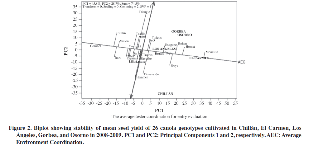
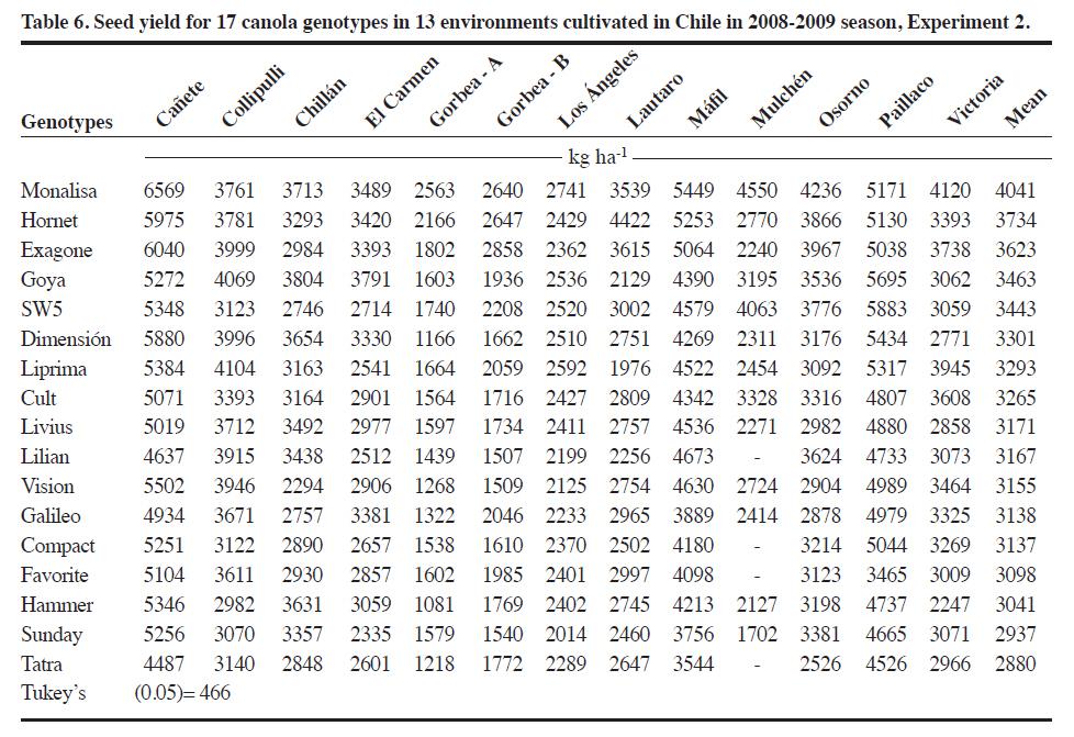
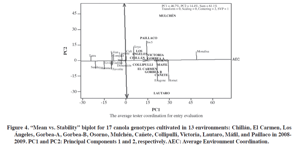
Experiment 1: 26 cultivars in five environments. The first two PCs explained 74.5% (PC1 = 45.8%, PC2 = 28.7%) of the total GGE variation with the centered model = 2 and SVP = 1. The proportion of the variation explained in this study (74.5%) was considered acceptable. Although it is not clear how much of the variation must be represented by the first two principal components involved in the biplot, recent publications indicate that at least both PCs must accumulate more than 60% of the variation generated by (G × GE) to interpret mega-environments with some validity (Yang et al., 2009). One explanation of this result was that all genotypes used are winter canola types with closely related pedigrees, and the genetic base for winter canola genotypes is also not very extensive, which may influence the G × E interaction (Long et al., 2007). The cvs. Rohan, Hornet, and Exagone were better adapted to the coldest and more humid southern environments, that is ‘Gorbea’ and ‘Osorno’, than to the hotter and drier northern location of Chillán where ‘Dimensión’ and ‘Hammer’ performed better. However, ‘Monalisa’ had the best seed yield in four of the five studied environments, and demonstrated the good seed yield stability of this genotype.To determine ‘which-won-where’, or which genotype is the best in which environment, an SREG analysis was conducted with a biplot as a visual tool. The GGE biplot is an effective visual tool to analyze mega-environments (Yan et al., 2000) consisting of an irregular polygon and a set of lines drawn from the biplot origin intersecting each of the sides at a right angle (Yan et al., 2007). The genotypes that are the farthest away from the biplot origin are located in the vertices of the polygon in different directions in such a way that all the studied genotypes are contained inside the polygon. The line running from the biplot origin intersects perpendicularly with the side of the polygon representing a hypothetical set of environments in which genotypes perform equally (Yan and Rajcan, 2002). If the studied environments are located in different sectors, this means that different genotypes obtained the highest seed yield in different environments (Yan et al., 2007). The biplot in Figure 1 is based on seed yields shown in Table 2. The five environments were located in two areas of the biplot marked by two different cultivars, and ‘Monalisa’ had the highest seed yield in all environments except Chillán. The lines perpendicular to the sides of the polygon divide the biplot into five sectors, but the five evaluated environments were located in only two of the areas or mega-environments. An interesting characteristic of the GGE biplot visualization is that cultivars in the vertices of the polygon are extreme cultivars with either the highest or lowest seed yield for each mega-environment made up of the original environments located in that area of the biplot (Yan et al., 2007). The Gorbea, Osorno, El Carmen, and Los Ángeles environments were grouped in one mega-environment with ‘Monalisa’ and ‘Hammer’ in the vertices of the polygon suggesting that these cultivars had the highest performance in these environments. The Chillán environment was located in a different area of the biplot with ‘Hammer’ and ‘Dimensión’ suggesting that they had a high performance. Interpretation of the biplot suggests that there are three possible outstanding cultivars, Monalisa, Goya,and Hornet for the mega-environment represented by Gorbea, Osorno, El Carmen, and Los Ángeles, as well as two cultivars in Chillán, ‘Dimensión’ and ‘Hammer’. Information generated in multiple years and environments is essential to decide if an environment or a region can be objectively divided into different mega-environments (Yan and Rajcan, 2002). Repeated locations are necessary, but not sufficient, to establish different mega-environments since cultivar response can change from year to year (Yan and Rajcan, 2002; Yan et al., 2007; 2009). Some authors have reported that the ‘which-won-where’ pattern is not repeatable in many cases, so that it is not possible to separate cultivation areas in real mega-environments (Navabi et al., 2006). To determine average potential performance and genotype stability, these factors were analyzed with the“Average Environment Coordination” method (AEC)(Yan, 2001; Yan and Rajcan, 2002; Yan et al., 2007). In this method, the average performance of environments is defined as the mean of PC1 and PC2 values of all environments represented by the small circle in Figure 2,and a single arrow line is drawn through the environment average and biplot origin. This AEC abscissa is the “average environment axis”. The AEC coordinate axis, AEC Y-axis, is the line that passes through the origin and is perpendicular to the AEC abscissa. Unlike the X-axis, which has a single direction towards the best cultivar, the Y-axis is indicated by the double arrow line. Genotypes located away from the AEC abscissa are less stable than those near the top or close to the AEC line. The Y-axis separates genotypes with lower and higher than average performance from the general genotype mean. Genotypes with a mean seed yield higher than the general mean for all genotypes were ‘SW5’,‘Tadeus’, ‘Dimensión’, ‘Brutus’, ‘Exagone’, ‘Goya’,‘Rohan’, ‘Hornet’, and ‘Monalisa’ whereas genotypes with a mean seed yield lower than the general mean were‘Hammer’, ‘Livius’, ‘Favorite’, ‘Taurus’, ‘Liprima’,‘Lilian’, ‘Sunday’, ‘Compact’, ‘Tassilo’, ‘Artus’, ‘Triangle’,‘Vision’, ‘Tatra’, ‘Cuillin’, and ‘Coronet’ (Figure 2). It is important to emphasize that this analysis method does not statistically differentiate genotypes and since hypothesis tests are not used in the analysis, conclusions are drawn by observing the biplot (Yang et al., 2009). On the other hand, genotype stability is important since it indicates if a high-yielding genotype in one environment maintains its relative ranking across environments. A very long line projected from the AEC coordinate, independent of its direction, represents a high G x E interaction. The mean of these genotypes can be more changeable in different environments and can then be considered as having lower stability. ‘Monalisa’ was the genotype with the highest stability and best performance (Figure 2). Genotypes in this study were classified according to the methodology suggested by Yan et al. (2007). Genotypes in the first group had the highest yield potential and high stability, and were therefore described as superior genotypes: ‘Monalisa’, ‘Hornet’, ‘Rohan’, ‘Exagone’, ‘Brutus’, ‘Goya’, and ‘SW5’. It must be emphasized that all cultivars in this group were hybrids except Goya. The second group included ‘Dimensión’ and ‘Tadeus’ with high yield potential, but low stability, that is, high seed yield only in some specific environments. The third group included cultivars with low seed yield potential, but high stability, a comparatively lower yield in all the evaluated environments and would therefore, not be recommended for any of the studied environments: ‘Coronet’, ‘Vision’, ‘Tatra’, ‘Compact’, ‘Galileo’, ‘Sunday’, ‘Liprima’, ‘Lilian’, ‘Taurus’, ‘Favorite’, and ‘Cult’. ‘Coronet’ was classified as low-yielding and highly stable. It is an old cultivar, early flowering and maturing, of lower height, biomass, and seed yield. All the cultivars classified in this group were open-pollinated except for ‘Lilian’ and ‘Taurus’, the latter being an old hybrid that will probably be promptly withdrawn from the market because of its susceptibility to Alternaria spp. The fourth group cultivars had low seed yield only in some of the environments: Tassilo, Triangle, Hammer, Artus, Cuillin, and Livius. Experiment 2: 17 cultivars in 13 environments. Combined ANOVA detected significant differences for environments (E), genotypes (G), and G × E interaction (Table 5). Of the total sum of squares of E + G + GG × E, 82.1% was the result of the environment, so that it is necessary to analyze how this factor influences the evaluated cultivars. The magnitude of the variation attributed to G × E also suggests the possibility of grouping environments in terms of the G× E interaction (Yan et al., 2000). These results coincided with those obtained in Experiment 1 (Table 6). The first two PCs explained 61.1% (PC1 = 46.7%, PC2 = 14.4%) of the total GGE variation with the centered model = 2 and SVP = 1. Analyzing these cultivars with only 61% of the total variation implies the risk of ignoring important aspects of the variation caused by G × E interaction. If we compare these results with those of the previous analysis with 26 cultivars and five environments, the ranking and grouping of cultivars in mega-environments, and the selection of high performance cultivars, they were similar. This is the main reason for discarding the G × E variation of 39% and not using the third PC in a 3-D biplot (Yang et al., 2009). In addition, other researchers, such as Kaya et al. (2006) and Roozeboom et al. (2008) also used only two PCs with accumulative variation of 62% for the construction of the GGE biplot in 25 cultivars of Triticum aestivum L. In order to visualize the same cultivar performance as in Experiment 1 in a greater number of environments, cultivar trial results from Agrosearch Ltda. were used in addition to the five studied environments. Experiments 1 and 2 were not combined into a single analysis because the variances were not homogeneous, and harvest and seed cleaning methods were different. The 17 cultivars evaluated in 13 environments were grouped in two sectors of the biplot with different superior cultivars on the vertices of the polygon (Figure 3). ‘Monalisa’ was the cultivar with the highest yield in 12 of the 13 environments and ‘Exagone’ and ‘Hornet’ had the highest yield only in the Lautaro environment. These results coincide with those from Experiment 1 in which ‘Monalisa’ had the highest yield in most environments. Figure 4 shows that the highest seed yield means were for ‘Goya’, ‘SW5’, ‘Exagone’, ‘Hornet’, and ‘Monalisa’, and the lowest means for ‘Cult’, ‘Liprima’, ‘Dimensión’, ‘Lilian’, ‘Compact’, ‘Favorite’, ‘Hornet’, ‘Sunday’, and ‘Tatra’. ‘Monalisa’ was the most stable and showed the highest performance. According to the results of this study during the 2008-2009 season, the ‘Monalisa’ hybrid showed the best seed yield potential in all environments with a high overall stability, which would classify it as a stable high performance cultivar. The cultivars with high seed yield in only some environments and low stability were SW5, Goya, Exagone, and Hornet. The cultivars with low seed yield potential in all environments were Vision, Dimensión, Liprima, Tatra, Livius, and Galileo. The cultivars in the fourth group that had a low seed yielding only some environments were Lilian, Favorite, Cult, Sunday, Vision, and Hammer. It is widely accepted that quantitative characters such as seed yield are controlled by multiple genes and their expression depends on the environment (Long et al., 2007). CONCLUSIONS It was concluded that seed yield in canola grown in Chile is strongly influenced by the genotype × environment interaction of the total variation. The environment and genotype × environment interaction were the most important with 65.8 and 14.5% of the variation, respectively, when evaluated in five environments, and 82.2 and 8.9% of the variation, respectively, in 13 environments. Of the 26 evaluated genotypes, six cultivars were well adapted to the environments of El Carmen, Los Ángeles,Gorbea A, and Osorno, as well as two which were better adapted to Chillán in the 2008-2009 season. In this study, ‘Monalisa’ had the highest seed yield and stability in most of the analyzed environments according to SREG analysis and GGE biplot. ‘Hornet’, ‘Goya’, and ‘Exagone’ also had an outstanding performance. According to the results, the cultivars most adapted to the canola production region of Chile would be the ‘Monalisa’, ‘Hornet’, and ‘Exagone’ hybrids, and the open-pollinated Goya cultivar. The conclusion is based on only 1 yr of experimentation,so that results could change if more data were included covering a longer period of time. ACKNOWLEDGEMENTS Funding for this research was provided by FIA (Fundación para la Innovación Agraria), project FIAPI-C-2007-1-A-008, Chile. Authors acknowledge the valuable collaboration of ALISUR S.A., Ricardo Montesinos Iroume, Molinera Gorbea Ltda., Biosemillas Ltda., Hernán Martínez Chavarría, and Waldo Cerón of Agrosearch Ltda. for providing 13more study sites. We also thank the technicians and students for plot planting, management, data collection, and analysis, especially Wilson González Saavedra and Alejandro Solis Fuentes. LITERATURE CITED
Copyright 2011 - Chilean Journal of Agricultural Research The following images related to this document are available:Photo images[cj11021t5.jpg] [cj11021f1.jpg] [cj11021f4.jpg] [cj11021t2.jpg] [cj11021t1.jpg] [cj11021t6.jpg] [cj11021f3.jpg] [cj11021t4.jpg] [cj11021f2.jpg] [cj11021t3.jpg] |
| |||||||||