+Bioline International Official Site (site up-dated regularly)

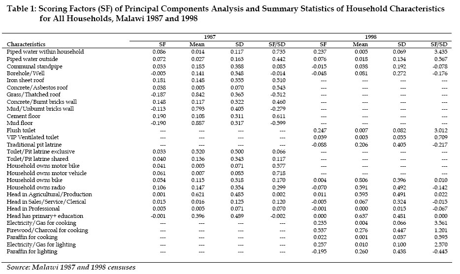
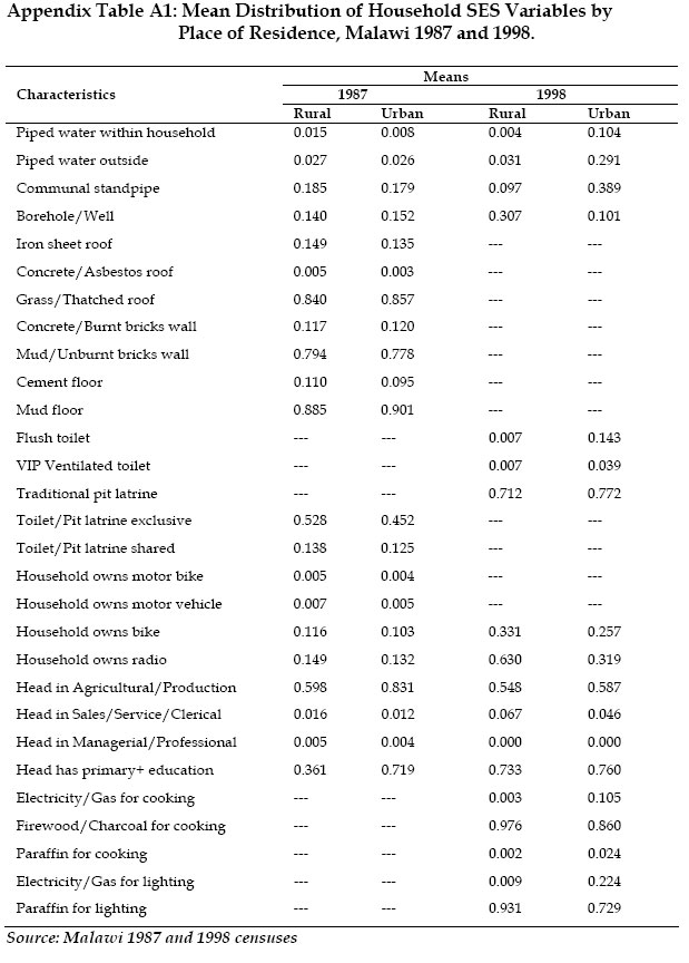
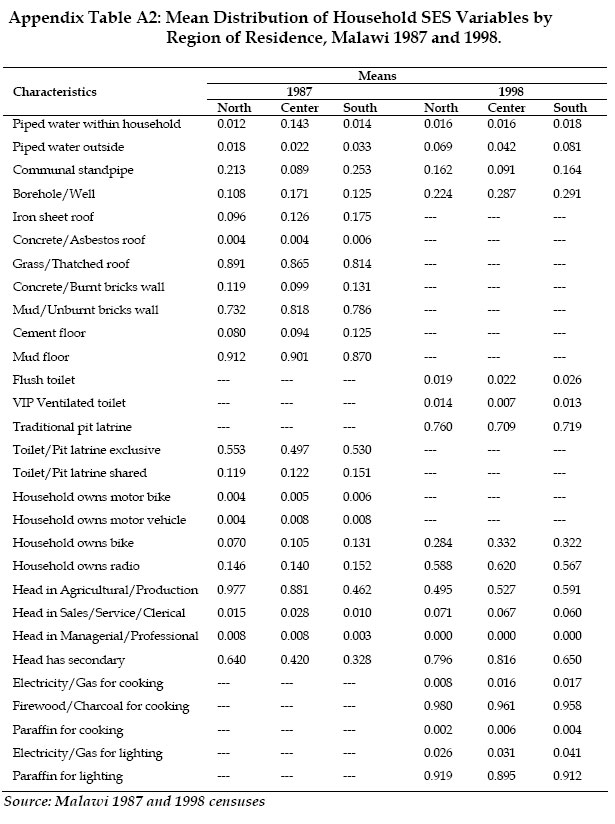
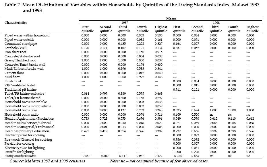
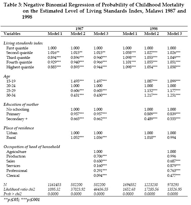
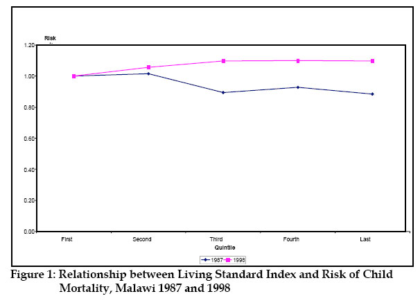
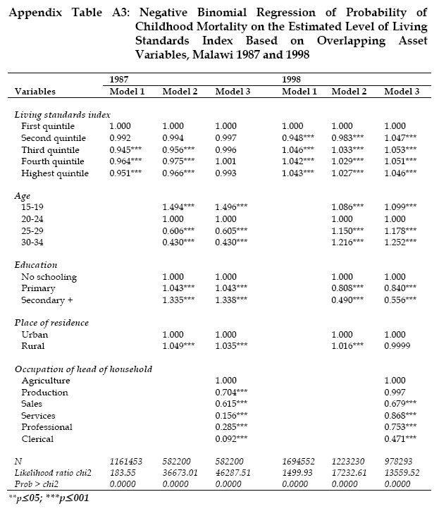
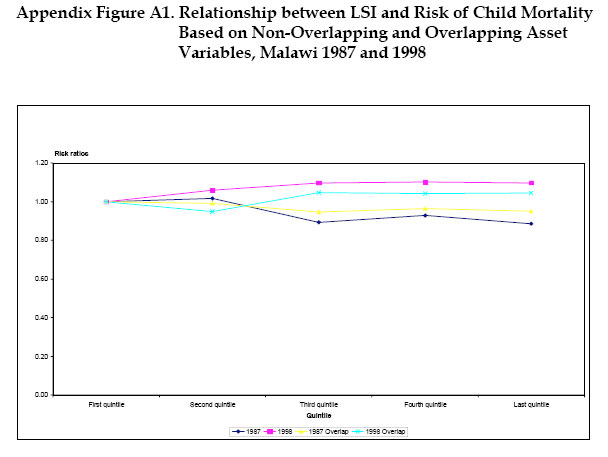
African Population Studies/Etude de la Population Africaine, Vol. 19, No. 2, Sup. A, 2004, pp.241-263

A number of studies have found that membership in a higher socioeconomic status (SES) group has a significant effect on different demographic outcomes such as lower infant and child mortality. Most of these studies have analyzed the association between SES and children’s survival by focusing on data on asset-ownership which includes, for example, owning a bicycle, radio or television; housing characteristics such as number of rooms or type of toilet facilities; and source of water. These household characteristics are conceived as having a direct or indirect role in shaping child mortality differentials. This paper uses principal components analysis to create a living standards index (LSI) based on the household characteristics and apply it in a multivariate model to examine its relationship with childhood mortality in Malawi using 1987 and 1998 census data. When the LSI is applied to the 1987 census data, the results show an increase in mortality for children who come from poor households. However, the results in 1998 differ from those in 1987 in that child mortality is higher among the rich households in 1998 and also among middle-aged women. These results are consistent with parallel analysis of the 1992 and 2000 Malawi Demographic and Health Survey data. We argue that based on the magnitude of the HIV/AIDS prevalence in Malawi and given the timing of the 1998 census in the stage of the AIDS epidemic, and also consistent with findings of high mortality in all households and high social class groups in Malawi, the shift in the effect of the LSI on child mortality may be attributed to this deadly disease.

Membership of a higher socioeconomic status (SES) (e.g., characterized by more education, higher income, urban residence, and better housing types) has a significant effect on different demographic outcomes such as lower infant and child survival (United Nations, 1985; Muhuri, 1996; Filmer and Pritchett, 2001). Most of these studies have analyzed the association between SES and children’s survival by focusing on data on asset-ownership which includes, for example, owning a bicycle, radio or television; housing characteristics such as number of rooms or type of toilet facilities; and source of water. These household characteristics are not only considered as asset indicators, but they are also conceived as having a role in shaping child mortality differentials in a country either directly or indirectly.

During the last decades, researchers have adopted different approaches in studying the relationship between SES and different demographic outcomes depending on their principal objectives and data availability. Because of the direct and indirect effects of SES on the demographic outcome variable, some researchers either present their analyses by examining the effect of each of the variables of interest separately, or treat them together as a proxy for SES by creating a composite index (Bawah, 2002).

A proxy for SES is not only useful in examining effects of wealth, but also is needed as a “control” variable in estimating effects of variables potentially correlated with household wealth, such as maternal education. The approach among researchers of using proxies for SES and creating a composite index arose as a result of the absence of either income or expenditure data. For example, income is not often used as a measure in developing countries because households frequently draw their income from multiple sources that can change from year to year and even from season to season. Hence it is a challenge for researchers to track these changes (Montgomery et al., 2000).

This paper uses a method consistent with other approaches (e.g., Filmer and Pritchett, 2001; Bawah, 2002) which use a combination of household variables such as roofing materials, wall materials, flooring materials, main source of drinking water, type of toilet facilities, household possessions, and source of energy as a proxy for SES. We then use them to create a living standards index (LSI) in a multivariate model to examine its relationship with childhood mortality in Malawi using the 1987 and 1998 census data. The objectives are: 1] to investigate how the level of the household’s SES affects the survival chances of the children, and 2] to find out whether between 1987 and 1998 levels of poverty changed in Malawi and the extent to which this change may have affected children’s survival chances. Another interest is to find out the variations in asset ownership by place of residence (rural/urban) in the two censuses.

In the context of Malawi, as is the case in other African countries, the idea of employing household characteristics as a proxy for SES to examine its relationship with mortality is not only prudent but also simple: the type of household characteristics and material possessions owned by the household are useful determinants of the health status of household members, particularly children, as well as indicators of the SES of households such as their purchasing power (Bawah 2002). Furthermore, the interest in this paper is to examine the combined effect of household characteristics (as an indicator of SES or living standards) and not the individual effect of the variables.

Measures of Socioeconomic Status

In the last decade, there has been an increasing use of information on demographic and socioeconomic characteristics of households by policymakers to formulate appropriate health policies for different countries. For example, household data can be used to determine the country’s needs and requirements for education and health infrastructure. However, the most important issue is to identify appropriate measures that convey meaningful information about the welfare of the household. For a number of years, researchers have measured SES at the national level based on incomes or consumption levels. A person is considered poor if his or her consumption or income level falls below some minimum level necessary to meet basic needs. This income is usually indexed by either the gross domestic product (GDP) or the gross national product (GNP). Although there has been continued use of the GDP and GNP, new directions in socioeconomic measurement show that these measures are flawed. At the micro-level, they are unable to assess the level of well-being at the individual or household level (Todaro 1978; Sen 1987).² While much progress has been made in measuring and analyzing income and poverty, efforts are needed to measure and study the many other dimensions of SES. There is a concern among researchers that some of these widely used measures do not capture the general well-being of the population (Bawah 2002). For example, although the GNP per capita helps to measure the material output of a country, it does not show what kinds of goods and services the country produces, whether all people share equally in the wealth of a country, or whether these people lead fulfilling lives.

Another measure, the Human Development Index (HDI) is often used as one of the measures of SES or development of a country. The HDI is a composite index that is a simple average of three indices reflecting a country’s achievement in terms of health and longevity. The indices are: 1] life expectancy at birth, 2] education (measured by adult literacy and combined primary, secondary, and tertiary enrollments), and 3] living standard (measured by GDP per capita in purchasing power parity³) (The World Bank, 2002). The advantage of the HDI is that it allows countries to be ranked in terms of their achievements in human development. The disadvantage, however, is that it does not allow the judgment of the relative importance of its different components, which change considerably over time. As discussed earlier, these macro measures are flawed in that they fail to account for variations at the micro-level.

Because of the need to understand the general well-being of individuals, several questions on household characteristics were collected in the less developed countries in censuses and surveys. For example, the World Fertility Survey (WFS), which was carried out between 1974 and 1984 in more than 40 countries, was a rich source of information in the developing world to be used for the analysis of household characteristics (De Vos, 1987). Similarly, the Demographic and Health Survey (DHS) program which began in 1984 as a follow-up to the WFS program, is the most recent source of information on household characteristics throughout the developing world (Ayad, Barrere and Otto, 1997). A number of African countries have collected information on some of these household variables and more specifically, in Malawi, information on household characteristics at the national level was first collected in the 1987 census followed by the 1998 census.

The basic idea behind information on household possessions is that households with piped water, flush toilets, a finished cement floor, roofing made from metal, using electricity for cooking, or those that possess a variety of consumer goods (ranging from a table, or a chair to a telephone, VCR, or a washing machine) are more likely to achieve good health status than those without these facilities or those that rely on surface water, pit latrines, rudimentary floors, etc. (Bawah, 2002). These household possessions are considered as indicating the level of affordability of good health services and some are markers of the capacity for personal hygiene.

A number of studies have examined the role of socioeconomic development as an important factor in mortality decline in historical countries of Europe (McKeown and Record, 1962). For example, McKeown, Record and Turner (1975) attributed the decline of mortality in England and Wales during the twentieth century to what they term “rising standards of living.” In addition, Haines (1995) using data from the 1911 census of the Fertility of Marriage of England and Wales studied patterns of mortality decline by socioeconomic characteristics, principally the occupation of the husband. The aggregate results showed that social class in England and Wales during the 1890s and 1900s tended to be related to the speed of mortality decline: childhood mortality declined more rapidly in the higher and more privileged social class groups. Overall, social class (or occupation group), income, and urbanization were more successful in explaining mortality levels than time trends across occupations, although social class and the extent of urbanization did reasonably well in accounting for trends.

In the developing world, similar results on the relationship between SES and child mortality have been found by a number of studies (e.g., Hobcraft, McDonald and Rutstein, 1984; United Nations, 1985; Cleland, Bicego and Fegan, 1992; Madise, 1996; Madise, Matthews and Margetts, 1999). For example, useful insights on the effect of SES (as measured by variables such as occupation status of mothers, income, and housing characteristics) on child survival were found by a 15-country study conducted by the United Nations (1985). These studies have demonstrated the importance of SES as a predictor of mortality since the latter is an outcome rather than a cause, and thus serves as a direct measure of the distribution and use of resources (Haines, 1995).

In the area of demographic and epidemiological research, the Mosley and Chen (1984) framework has most influenced public policy through their view of “distal” socioeconomic factors such as education and income as factors influencing disease incidence and outcomes as measured by five broad groups of “proximate” determinants of child survival: maternal factors, nutrient deficiency, environmental contamination, injury, and personal illness control. The last one includes both the availability of health services and the capacity to use them (Lopez, 2000). The proximate determinants perspective views mortality as an endpoint that is influenced by biomedical and socioeconomic factors and implies the need for an integrated approach to the study of child health and mortality.

Bawah (2002) points out that an examination of the effects of biomedical or biological factors on child health requires direct measurement of these factors in the field—which is often not possible. These factors can be identified by anthropometric measures such as weight of children, height, and upper arm circumference, and in some cases blood samples to measure hemoglobin levels. Most social surveys do not collect this information since social and economic factors are easier to collect and serve as proxies for measuring the determinants or factors related to child’s growth.

Although this paper examines the relationship between the type of housing characteristics and household possessions as proxies for SES of the household (and its effect on child mortality), this discussion cannot be complete without warning that the extremely high HIV/AIDS prevalence in Malawi may bias the effect of living standards on child mortality. The HIV/AIDS epidemic has an enormous impact first on adult mortality, and subsequently on child survival (Lopez, 2000). In other parts of southern Africa where adult HIV seroprevalence is around 20%, there is already evidence of an increase in child mortality. This indicates a threat to child survival in Malawi where HIV is spreading rapidly and progress in reducing child mortality has been comparatively modest. Although this paper is not about the impact of HIV/AIDS on child mortality, it is reasonable to acknowledge that HIV/AIDS still remains a challenge in most economic analysis of child survival in Malawi.

Data for analysis come from the 1987 and 1998 Malawi censuses. The 1987 census includes information on 38 asset indicators that can be grouped into two types: 1] characteristics of the household’s dwelling with 33 indicators (eight about sources of drinking water, six about toilet facilities, six about roofing facilities, seven about wall materials, one question on number of rooms, and five about flooring materials); and 2] household ownership of consumer durables with five questions (radio, bicycle, motorcycle, motor vehicle, and ox-cart).

The 1998 census includes less information and collected a total of 26 asset indicators with the first grouping similar to the 1987 census and consisting of 10 questions about sources of drinking water, four about toilet facilities, and nine about sources of energy. The last group of household possessions had three items only (ownership of radio, bicycle, and ox-cart). Only 20 asset indicators are overlapping in the two census years and these include seven about sources of drinking water, one about toilet facility, and three about household durables. All these asset indicators are reduced by combining some of them thus bringing to the total to 39, that is, 21 asset indicators for 1987 and 18 for 1998.

The 1987 and 1998 Malawi censuses also collected information on individual-level characteristics such as education and economic activity (occupation). More important is the information that can be used to examine child survival such as the number of children ever born to women aged 10 years or more (1987 census) or 12 years or more (1998 census) and the number of children dead.

The Malawi census data are obtained from the archives of The African Census Analysis Project based at the University on Pennsylvania, Population Studies Center (http://www.acap.upenn.edu). These data are used to create a composite household LSI and investigate its effect on child mortality in Malawi in 1987 and 1998.

With the information available in the census data, the question still remains: how does one aggregate different asset indicators into one variable to proxy for household “wealth”? Even if the question is simplified by limiting the aggregation to a linear index, how should the weights (or the different contributions of the variables) be chosen? It has been argued by others (e.g., Duncan, 1984) that the problem associated with creating a composite index is next to impossible to solve since this involves combining “intrinsically heterogeneous components.”

In the past, researchers have proposed and used different approaches to developing a composite index (Bawah, 2002). One plausible option has been not to build an index at all but simply to enter all of the asset variables separately in a linear multivariate regression equation. Although this procedure implicitly creates weights on the variables, the linear index of the assets using regression weights does not estimate the wealth effect because many assets exert both a direct and indirect effect on the dependent variable. For instance, the household’s use of electricity for lighting may serve as a proxy for wealth, but may also make study easier and hence lower the opportunity costs of schooling. Another example is the availability of piped water which not only indicates greater wealth but also may reduce the time needed for collecting water and thus may reduce the opportunity costs of schooling. This argument is clearer with health outcomes than with schooling outcomes because water and sanitation have strong independent effects on children’s health (Filmer and Pritchett, 2001). Therefore, while the use of such a procedure implicitly produces weights for the linear index of the asset variables that closely predict the outcome variable, there is no way to infer from these unconstrained coefficients the impact of an increase in assets (Filmer and Pritchett, 2001).

Other approaches that have been suggested range from one extreme of creating a simple index by assigning equal weights to the variables used in the index, to the other extreme where each variable is considered as a covariate in a regression model which implicitly weights the variable (Bawah, 2002). A straightforward and pragmatic statistical procedure called principal components analysis (PCA)⁴ has been used for a considerable time to determine the weights for an index of the assets variable (Dunteman, 1989; Filmer and Pritchett, 2001; and StataCorp, 2001).

Armed with data on child mortality (children dead) from the census on the one hand, and the LSI on the other, we examine how child mortality differs in Malawi according to the household’s living standard. We hypothesize that mortality is likely to be higher in “poorer” than in “richer” households. Negative binomial regression is used because we observe the number of children (³0) who have died out of those ever borne by women.⁵ The negative binomial model also includes an offset term which adjusts for exposure and its coefficient is constrained to one. Consistent with other approaches (Das Gupta, 1997; Bawah, 2002), we use children ever born as an offset term. This variable accounts for the effect of fertility and duration of exposure since the risk of mortality for children depends on the number of children who are already born. The estimated negative binomial model will adopt the maximum likelihood regression.

Table 1 presents the scoring factors (SF) from the PCA of the household asset variables from the 1987 and 1998 census data. Each variable is dichotomous, making its mean and standard variable deviation range between 0 and 1. As noted earlier, there are some variables that are unique to each year.⁶ The observed pattern in the first (SF) column of each year is consistent with our expectation: higher positive scores are assigned to variables that are more likely to be associated with richer households and low or negative values are more likely to be associated with poor households. For instance, positive values are assigned to piped water inside house, iron sheets, motor vehicle, cement floor, etc. On the other hand, low or negative values are assigned to traditional pit latrine, grass/thatched roof, borehole/well, etc. Because these variables are dichotomous, the weights have an easy interpretation: a move from 0 to 1 (i.e., a move from “no ownership” to “owning” an asset) changes the index by the amount of SF/SD (ratio of scoring factor to standard deviation—column four of each year). For example, in 1987 and 1998, a household that has piped water inside the house has an asset index higher by 0.735 and 3.435 respectively than one that does not have piped water inside. Owning a bicycle raises a household’s asset index by 0.054 in 1987 and 0.004 in 1998. The distribution of the remaining variables can be interpreted in a similar manner.

The number of households having access to certain assets that are comparable between 1987 and 1998 shows that on average there has been either an increase or a decrease in access to those assets between the two censuses. For example, in Table 1, 11.5% of households owned bicycles and this proportion rose to 80.6% in 1998. About 14% had access to water from a borehole in 1987 whereas in 1998 this proportion declined to a low of 8.1%. 40% of household heads had at least primary education in 1987 whereas in 1998 this proportion rose to 64%. Similar analysis was done for the 20 overlapping asset indicators which are reduced to 10 and the results (not reported here) are consistent with those obtained in Table 1in terms of the magnitude of the scoring factors.

The mean distribution of household SES by place of residence is provided in Appendix Table A1. For household assets that are comparable between 1987 and 1998, the results are similar to those reported in Table 1; that is, there has been an increase or a decrease in the proportion of households owning certain assets over the 11-year period. This finding (i.e., increase or decrease in assets) is also true on average for the urban areas. Regional variations in asset ownership are provided in Appendix Table A2. The distribution of variables in 1987 and 1998 shows similar patterns between the census years and for each region as reported in Table 1 and Appendix Table A1.

A surprising finding, however, is the distribution of the variables across quintiles in 1998. The distribution for all variables except the household durables is concentrated in the first two quintiles of the LSI which implies that the differences between the quintiles are small. The LSI on average ranges from –0.567 units among the lowest 20% of the households to 2.427 units among the highest 20% in 1987 whereas in 1998 it ranges from –0.285 among the lowest 20% of the households to 0.658 among the households in the second quintile.⁷ The difference in the average index between the richest 20% and the poorest 20% of the households is 2.994 (i.e., 2.427–(–0.567)) for 1987 and 0.943 (i.e., 0.658–(–0.285)) in 1998 suggesting that the differences between the poor and rich is growing smaller over time. The reader is reminded here that the classification of “richest” and “poorest” households does not follow any of the usual definitions of poverty but is based on the scoring factors obtained from PCA (see Sahn and Stifel 2000; Filmer and Pritchett 2001).

Multivariate Analysis of Living Standards on Child Mortality

To assess the effect of different levels of living standards, we estimate a separate negative binomial regression model of child mortality on living standards based on the quintiles for each census year and in separate models control for other variables such as age and education of the mother, place of residence, and occupation of head of household. And as indicated earlier, we expect child mortality to be lowest in rich compared to poor households and the differences between the rich and poor households should be stronger in 1998 than in 1987.

To assess the relationship between LSI and child mortality, we ran three separate models for 1987 and 1998 with the number of children dead as the outcome variable and LSI as the main predictor variable of interest. Results of these analyses are presented in Table 3. The first model of each year only considers the baseline effect of the LSI on the index of child mortality at the household level. In model 2 we add age, education of the mother, and place of residence whereas model 3 finally adds the occupation of the head of household.

The total effect of LSI on child mortality shows that in 1987 mortality declines with the level of LSI, that is, as we move from the lowest quintile to the highest quintile, the risk of mortality is reduced (p<.001). For example, model 1 in 1987 shows that the risk of mortality is reduced by 7% in the fourth quintile and further reduced by 12% in the highest quintile. In model 2 of 1987, after controlling for age, education, and place of residence, the risk of mortality is reduced as we move toward the high levels of LSI. In addition, we see that the risk of mortality increases for young mothers compared to those aged 20–24. Child mortality is low for mothers who are older. For example, the risk of mortality declines by about 39% and 56% for women aged 25–29 and 30–34 respectively. The effect of education on child mortality shows lower mortality for children whose mothers are educated than those who are not. The risk of mortality is also higher for people in the rural areas than their urban counterparts. In model 3 of 1987, the effect of LSI on child mortality is still robust and maintains the same direction, that is, lower mortality as we move from poor to rich quintiles. The risk ratios after controlling for the other variables are similar to model 2. Occupation of the head of household has a significant effect on child mortality. When the head of household is in the production category, mortality is reduced by about 29% and further reduced by about 37% for those engaged in sales compared to those in agriculture. Those who do service work experience about 84% reduction in child mortality. Professionals and clerks have a 71% and 91% reduction in child mortality respectively.

Although the baseline effect of LSI on child mortality is significant in 1998, the results are contrary to what one would predict. Mortality is about 6% higher among households in the second quintile than those in the first quintile and the risk increases to about 10% as we move toward the highest quintile. In model 2 when we control for age, education, and place of residence, the results show that the effect of the LSI is still robust and in the same direction as in the baseline model. However, child mortality is higher among almost all women which is contrary to the results in 1987. This result is persistent: in models 2 and 3, children of older mothers experience high mortality whereas children of highly educated women have low mortality. Although people in the occupations considered better off than those in the agricultural category experience a reduction in the risk of child mortality, the reduction is less than that observed in 1987. These results suggest that in 1998, mortality is concentrated in the richest households and this is also consistent with (1) the results of the baseline effect of LSI on child mortality, and (2) findings from other surveys such as the Malawi 2000 DHS (National Statistical Office [Malawi] and ORC Macro 2001) that have found increased mortality among households in Malawi (apparently due to HIV/AIDS) irrespective of the level of SES.⁸

The relationship between mortality risk ratios and the LSI (model 1 only) for the two censuses is displayed in Figure 1.

For 1987, the graph shows a negative relationship between childhood mortality and living standards. The chances of survival are higher among households in the higher level of SES than those in the lower levels of the LSI. The 1998 results show an increase in the risk of mortality between the SES groups.

Although there are no data in this study to explain the unexpected distortion in the effect of the LSI on child mortality in 1998, these results might suggest the impact of HIV/AIDS on the mortality pattern. The HIV/AIDS epidemic has an enormous impact first on adult mortality and subsequently on child survival (Lopez 2000). The adult HIV seroprevalence in Malawi is about 15% (UNAIDS 2003) and there is already evidence of an increase in child mortality between 1992 and 2000 apparently due to HIV/AIDS (National Statistical Office [Malawi] and ORC Macro 2001). If HIV/AIDS is a probable candidate in the observed distortion, then the results are in the expected direction. For example, if AIDS mostly affects the rich households—because they have resources that may initiate risky behaviors,⁹ e.g., having sex with prostitutes or other partners—then in the absence of antiretroviral drugs, any children born to women (who are infected) would eventually die due to the associated effects of HIV/AIDS such as loss of income and degrading health. In addition, HIV/AIDS prevalence is high in the prime age groups (15–50) and one would expect that children born to HIV+ women in this age range would have a high probability of dying.

The results reported so far are based on the household asset indicators that are different (non-overlapping) for the two census years. In order to find out whether the estimates obtained using the LSI based on the non-overlapping asset variables and the LSI based on the overlapping asset variables are consistent, separate analyses are presented in Appendix Table A3. Results show that there are no huge differences in the magnitude of the estimates in the two censuses. A summary of Appendix Table A3 is displayed in Appendix Figure A1 which shows a near-overlap in the curves for both census years.

Discussion

In this chapter, the relationship between living standards and child mortality has been estimated without income or expenditure data but instead by using household asset variables. Principal components analysis provides plausible weights for an index of assets to serve as a proxy for SES or wealth. An index of living standards was created and households were categorized into five social status or poverty groups and then the relationship between these groups and child mortality was explored. In Malawi, this approach produces meaningful results (at least for 1987), which are consistent with earlier studies on the negative association between wealth and child mortality (e.g., Das Gupta 1997; Bawah 2002). When the asset index is applied to the 1987 census data, the results show an increase in mortality for children who come from poor households. However, the results in 1998 differ from those in 1987 in that child mortality is higher among the rich households in 1998 and also among middle-aged women. We argue that based on the magnitude of the HIV/AIDS prevalence in Malawi and given the timing of the 1998 census in the stage of the AIDS epidemic, and also consistent with findings of high mortality in all households and high social class groups in Malawi (Bollinger, Stover, and Palamuleni 2000; National Statistical Office [Malawi] and ORC Macro 2001; Harries et al. 2002; National AIDS Commission [Malawi] 2003), the shift in the effect of the LSI on child mortality may be attributed to this deadly disease. In brief, these studies confirm the fact that AIDS has had (and is still having) serious economic impact on households. The epidemic is expected to increase the death rate at all ages with the most severe impact observed among adults in the prime working ages and among children under age 5.

The results of this study suggest that in African populations such as Malawi, where information on income or other direct measures of SES are scarce, employing information on household characteristics can provide researchers with valuable insights into other socioeconomic outcomes such as morbidity, utilization of health facilities, fertility, and contraceptive use.

The kind of analysis employed in this paper often raises questions about the suitability of the composite index of living standards as it relates to child mortality; that is, what is the differential contribution of the individual variables in creating the living standards index. The most important thing to remember is that the variables used in the analysis are viewed in their role as a proxy for SES. The index is not conceptualized as representing the individual effect of these variables on mortality but as a proxy for income. Although the index is weak in capturing the effects of the two key determinants of modern mortality improvements, that is, improvements driven by individual behavior—such as good nutrition as a result of rising income (McKeown, Record, and Turner 1975)—and changes driven by public health measures, this index captures the combined effect of these two key determinants at least in settings with limited data on income measures.

Notes

1. At the time this research was conducted, the author was a doctoral candidate in demography at the University of Pennsylvania, Philadelphia, USA.

2. Although these measures are deemed flawed to some extent, other research indicates that inequality in income distribution in a nation, state, region, or community is associated with higher morbidity and mortality rates, over and above the impact of the average socioeconomic level (e.g., Robert, 1999 and references therein).

3. Purchasing power parity (PPP) is a theory that states that exchange rates between currencies are in equilibrium when their purchasing power is the same in each of the two countries. This means that the exchange rate between two countries should equal the ratio of the two countries' price level of a fixed basket of goods and services. When a country's domestic price level is increasing (i.e., a country experiences inflation), that country's exchange rate must depreciate in order to return to PPP (http://fx.sauder.ubc.ca/PPP.html); accessed 2 June 2004.

4. Principal components analysis is a statistical technique for data reduction. The method helps the researcher to reduce the number of variables in an analysis by describing linear combinations of the variables that contain most of the information in the original variables (see Dunteman, 1989 and StataCorp, 2001 for a detailed description).

5. In this model, the dependent variable is believed to be generated by a Poisson-like process that accounts for unobserved heterogeneity, except that the variation is greater than that of a true Poisson. This extra variation is referred to as overdispersion (Allison, 1999) and can arise when the model is not well specified (missing variables), there are outstanding outliers, or the independence assumptions of the Poisson counts are violated. Poisson’s major property is that for any given set of covariates, the variance of the outcome variable is equal to its mean. The problem with this property is that it does not behave like this in practice since the variance tends to exceed the mean. In addition, the Poisson model does not account for the effect of unobserved heterogeneity and this leads to overdispersion. When overdispersion is present, standard errors are biased leading to an inflation of test statistics and widening of confidence intervals. A way to circumvent this problem is to model the negative binomial model by including an error term that accounts for unobserved heterogeneity (Allison 1999). The advantage of the error term is that it captures the unobserved variables that have not been included in the specified model. In addition, the error term is independent of the measured variables and also has a standard logistic distribution. For further details about estimation of negative binomial regression see Allison (1999).

6. Although the LSIs have different components in the two years (based on the unique variables), we still can compare the top and bottom quintiles between the two years. It all depends on how one interprets these changes. If one is comparing child mortality (as is the case in this chapter) in the top and bottom quintiles in the two years, as long as one thinks that the asset index is reasonable (and we do think so) in each year, one is justified in making statements like “child mortality in the top quintile has gone down” and so on. What is unknown, however, is whether the average standard of living (or to be simple, income) has gone up or down for this group. These statements are made relative to other people in the same year—albeit fixing the part of the distribution we are looking at in the two years. Further, we present our analysis based on overlapping and non-overlapping assets in the two censuses and this provides some leverage for our comparison.

7. These values have been standardized to mean zero and variance one.

8. We compared the findings from the census data with those from the Malawi 1992 and 2000 DHS. The results are the same: child mortality is higher among rich households in 2000 than it was in 1992.

9. This is the case in Malawi as reported in Harries et al. (2002) who found high AIDS- and Tuberulosis-related deaths among the rich and highly educated. Ankrah (1991) reports that AIDS is called a disease of poverty. Poverty causes work migration and urban drift, and it causes women to engage in risky sexual practices.

References

Allison, P. 1999. Logistic Regression Using the SAS System. NC: Cary, USA.
Ankrah, E.M. 1991. “AIDS and the Social Side of Health.” Social Science and Medicine 32, (9): 967-980.
Ayad, M., Barrere, B. and Otto, J. 1997. Demographic and Socioeconomic Characteristics of Households. Calverton, MD. Macro International Inc.
Bawah, A.A. 2002. Health, Well-being, and Mortality in Africa. Ph.D. dissertation in Demography, University of Pennsylvania.
Bollinger, L., Stover, J. and Palamuleni, M.E. 2000. The Economic Impact of AIDS in Malawi.
Washington DC and North Carolina: The Futures Group International, Research Triangle Institute, and The Centre for Development and Population Activities.
Cleland, J., Bicego, G. and Fegan, G. 1992. “Socioeconomic Inequalities in Childhood Mortality: The 1970s to the 1980s.” Health Transition Review 2, (1): 1–18.
Das Gupta, M. 1997. “Socio-Economic Status and Clustering of Child Deaths in Rural Punjab.” Population Studies 51, (2): 191–202.
De Vos, S. 1987. “Latin American Households in Comparative Perspective.” Population Studies 41, (3): 501–517.
Duncan, O.D. 1984. Notes on Social Measurement: Historical and Critical. New York: Russell Sage Foundation.
Dunteman, G.H. 1989. Principal Components Analysis. Quantitative Application in the Social Sciences, No. 69.
Filmer, D. and L.H. Pritchett. 2001. “Estimating Wealth Effects Without Expenditure Data--Or Tears: An Application to Educational Enrollments in States of India.” Demography 38, (1): 115–132.
Haines, M.R. 1995. “Socio-Economic Differentials in Infant and Child Mortality During Mortality Decline: England and Wales, 1890–1911.” Population Studies 49: 297–315.
Harries, A.D., N.J. Hargreaves, F. Gausi, J.H. Kwanjana, and F.M. Salaniponi. 2002. “High Death Rates in Health Care Workers and Teachers in Malawi.” Transactions of the Royal Society of Tropical Medicine and Hygiene 96, (1): 34-37.
Hobcraft, J.N., J.W. McDonald, and S.O. Rutstein. 1984. “Socio-economic Factors in Infant and Child Mortality: A Cross-National Comparison.” Population Studies 38:193– 223.
Lopez, A.D. 2000. “Reducing Child Mortality.” Bulletin of the World Health Organization 78, (10): 1173.
Madise, N.J., Z. Matthews, and B. Margetts. 1999. “Heterogeneity of Child Nutritional Status between Households: A Comparison of Six Sub-Saharan African Countries.” Population Studies 53: 331–343.
Madise, N.J. 1996. “Child Mortality in Malawi: Further Evidence of Death Clustering Within Families.” Pp. 27–35 in Population Dynamics: Some Past and Emerging Issues, edited by R.A. Powell, E. A. Mwageni, and A. Ankomah. Exeter, England: University of Exeter, Institute of Population Studies.
McKeown, T., R.G. Record, and R.D. Turner. 1975. “An Interpretation of the Decline of Mortality in England and Wales During the Twentieth Century.” Population studies 29, (3): 391–422.
McKeown, T. and R.G. Record. 1962. “Reasons for the Decline of Mortality in England and Wales During the Nineteenth Century.” Population Studies 16, (2): 94–122
Montgomery, M.R., M. Gragnolati, K.A. Burke, and E. Paredes. 2000. “Measuring Living Standards with Proxy Variables.” Demography 37, (2): 155–174.
Mosley, W.H. and L.C. Chen. 1984. “An Analytical Framework for the Study of Child Survival in Developing Countries.” Population and Development Review 10, (Supplement): 15–45.
Muhuri, P.K. 1996. “Estimating Seasonality Effects on Child Mortality in Matlab, Bangladesh.” Demography 33, (1): 86–110.
National AIDS Commission [Malawi]. 2003. HIV/AIDS in Malawi: Estimates of the prevalence of infections and the implications. Lilongwe, Malawi: National AIDS Commission.
National Statistical Office [Malawi] and ORC Macro. 2001. Malawi Demographic and Health Survey 2000. Zomba, Malawi and Calverton, MD: National Statistical Office and ORC Macro.
Robert, S.A. 1999. “Socioeconomic Position and Health: The Independent Contribution of Community Socioeconomic Context.” Annual Review of Sociology 25: 489–516.
Sahn, D.E. and D.C. Stifel. 2000. “Poverty Comparisons Over Time and Across Countries in Africa.” World Development 28, (12): 2123–2155.
Sen, A.K. 1987. The Standard of Living. Cambridge: Cambridge University Press.
StataCorp. 2001. Stata Statistical Software: Release 7.0. College Station, TX: Stata Corporation.
StataCorp. 1999. Stata Statistical Software: Release 6.0. College Station, TX: Stata Corporation.
The Joint UN Programme on HIV/AIDS [UNAIDS]. 2003. AIDS Epidemic Update: December 2003. http://www.unaids.org/html/pub/publications/irc-pub06/jc943-epiupdate2003_en_pdf.pdf; accessed 2 June 2004.
The World Bank. 2002. “Composite Indicators of Development.” http://www.worldbank.org/depweb/beyond/beyondco/beg_15.pdf; accessed 16 July 2002.
Todaro, M.P. 1978. Economic Development in the Third World. London: Longman.
United Nations. 1985. Socioeconomic Differentials in Child Mortality in Developing Countries, ST/ESA/SER. A/97. New York.

Measures of Socioeconomic Status

The following images related to this document are available:

Photo images