African Population Studies/Etude de la Population Africaine, Vol. 19, No. 2, Sup. B, 2004, pp. 9-29

Socioeconomic Status and Child Mortality: An Illustration Using Housing and Household Characteristics from African Census Data

Ayaga A. Bawah, and  Tukufu Zuberi

Population Council Postdoctoral Fellow, Ghana.   
Professor of Sociology, University of Pennsylvania, U.S.A  

Code Number: ep04033

ABSTRACT

Housing characteristics and household possessions such as sources of water; type of toilet facilities; housing construction materials; and household possessions like radio, television, and animal possessions, often reflect the socioeconomic status of households, especially in developing countries where income data are lacking. It is possible therefore, to use these variables together or individually to proxy for household wealth or socioeconomic status. This is because the type of houses people reside in and their possessions tend to speak to their economic ability or purchasing power. We treat the variables together as a proxy for economic status to create a composite poverty index and employed this index in multivariate model to examine its association with childhood mortality in three southern African countries. The results are reassuringly consistent with expectation, both simply by examining the mean distribution of the variables by the socioeconomic groups and also by the relationship of the index to childhood mortality in a multivariate regression model. The chances of childhood mortality decreased consistently with higher levels of the socioeconomic status index.

 INTRODUCTION  

The demographic literature is replete with studies demonstrating the significance of household characteristics and possessions on different demographic outcomes (Hobcraft, McDonald and Rutstein, 1984; United Nations, 1985; Cleland and van Ginneken, 1988; Sastry, 1996; Muhuri, 1996; Ayad, Barrère and Otto, 1997; Montgomeryet al., 2000; Filmer and Pritchett, 2001). In many of these studies, household characteristics such as source of water; type of toilet facilities; housing construction materials; and household possessions like radio, television, and animals are either conceived as indicators of economic status (and could therefore influence demographic outcomes indirectly) or are thought to have direct effect, such as, for example, water and toilet facilities on mortality. Different researchers have adopted various approaches in their use of these variables for demographic analysis depending on their conceptualization of the relationship between the particular variable and the outcome of interest. Because of the possibility of dual roles (direct and indirect effects on the outcome variable), some researchers either examine the effect of each of the variables separately or treat them together as mimicking socioeconomic status by creating a composite index.

In this paper, we treat these variables together as a proxy for economic status and therefore use them to create a poverty index and subsequently employ this index in a multivariate model to examine its association with childhood mortality in three southern African countries. Our conceptualization is based on the fact that the level of socioeconomic status does make a difference in terms of child survival and since for most of these countries we do not have credible income data (which are often used as a measure of socioeconomic status), we could use these variables as proxies for socioeconomic status. The reason is simple: in Africa, the type of household that one lives in and material possessions owned by the household speak to the economic status of members of the household in terms of their economic abilities or purchasing power. It should be noted at the outset that our interest is not so much in the direct effect of each of the variables as it is in their combined effect as reflecting economic status.

BACKGROUND

Traditionally, socioeconomic status at the national level is measured by the level of income indexed crudely by either the gross domestic product (GDP) or gross national product (GNP). However, these measures have historically been found to be problematic in measuring economic status at the micro-level because of their inability to capture adequately the notion of well-being at the individual or household level (Todaro, 1978; Sen, 1987; Mazumdar, 1999). The use of per capita gross national product (GNP) as an indicator of human well-being, for example, was discovered in the 1960s to be inadequate, leading to a redefinition of well-being by economists and development theorists to include poverty reduction, reduced inequality, and decrease in unemployment (Todaro, 1978). Sen (1985; 1987 and 1992) has argued repeatedly that measures of standard of living must capture happiness, utility, and choice; the ultimate objective being to enhance the well-being of people. He has particularly been very critical of the undue emphasis on income as a measure of well-being and instead advocated a basic needs approach using social indicators such as freedom of choice, the quality of the physical environment, etc. The United Nations (UNDP, 1990) also suggested the use of a human development index (HDI), which in principle also emphasizes the basic needs approach. In particular, the HDI places emphasis on human longevity as reflected in life expectancy, acquisition of knowledge in terms of level of literacy, and access to resources for a decent standard of living (UNDP, 1990).

In line with the principles of the basic needs or human well-being approach, various questions on household characteristics or possessions conceptualized to reflect socioeconomic status were included in the 1970 round of censuses and subsequently, with the hope that these will help measure differences in the level of socioeconomic status among households in different countries (United Nations, 1985). Recently, the World Bank has also started conducting what they term Living Standard Surveys (http://www.worldbank.org/html/prdhp/lsms/lsmshome.html) in several developing countries modelled along lines similar to those of the census modules with the aim of capturing information that could give indications on socioeconomic well-being in countries where income data are either not available or are unreliable.

The basic idea is that households with pipe-borne water; water closet (WC)/flush toilet; electricity for cooking or lighting energy; such durable consumer items as TV, radio, and animals; and are constructed with “modern” materials are likely to be “richer” than those without these facilities or those that rely on public toilet or use water from public sources, wells, rivers, and other community sources, etc.  This is because in many cases possessing these facilities reflects the household’s ability to afford them (although ability can be constrained in some cases because the basic infrastructure does not exist in the community, one of the methodological constraints we shall be discussing). It is possible then to use these variables, either individually or as an aggregate, to differentiate households on the basis of their level of economic well-being.

A number of African censuses have collected information on some of these household-level variables, in addition to individual-level characteristics. The information collected usually includes such individual-level characteristics as education and occupation of household members and their sex, and such household- or community-level variables as place of residence; type of building materials; availability of electricity; source of drinking water; type of toilet facilities; type of cooking fuel; and possession of certain household items such as television, radio, and animals (e.g., cattle, sheep, goats,). Information is also collected on the classic Brass-type questions—the number of children ever born, those who are dead, and/or those still surviving to women reported in the household. We use information from the 1991 population census of Botswana, the 1996 Lesotho census and the 1990 census of Zambia archived by the African Census Analysis Project (http://www.acap.upenn.edu) to create a composite index of living standards or poverty and examine the association between this index and childhood mortality in the three countries. We do not intend to compare the indexes across the three countries because of possible differences in the definition of the variables and due to the fact that some variables are specific to some countries.

Theoretical Perspective

The level of socioeconomic development has been recognized to play a critical role in mortality decline in historical Europe (McKweon and Record, 1962; McKweon, Record and Turner, 1975; McKweon, 1976). In their famous article “An interpretation of the decline of mortality in England and Wales during the twentieth century,” McKweon, Record, and Turner (1975) attributed the decline to “rising standards of living” (p. 391). As in the case of historical Europe, studies in developing countries have also demonstrated the effect of socioeconomic status variables on childhood mortality (Tabutin and Akoto, 1992; Cleland and van Ginneken, 1988; Hobcraft, McDonald and Rutstein, 1984; United Nations, 1985). For instance, in a detailed and elaborate 15-country study the United Nations (1985) demonstrated a positive association between socioeconomic status variables such as income, work status of mothers, characteristics of housing, including toilet and water supply facilities, and child survival in developing countries.

Mosley and Chen (1984) elaborated a conceptual framework articulating the relationship between socioeconomic and biomedical factors on child health and mortality. The novelty of the proximate determinants framework suggested by Mosley and Chen is that mortality, as an endpoint, is influenced by both biomedical and socioeconomic factors, suggesting an integrated approach to the study of child health and survival.  Unfortunately, examining the effects of the biological or biomedical factors on child health often requires direct measurement of these factors in the field. For example, we can estimate the effects of malnutrition by using anthropometric measures such as taking weights of children, measuring their heights and upper arm circumferences, and in some cases taking blood samples to measure hemoglobin levels. On the other hand, in the social sciences it is relatively easier to collect information on the social and economic background of respondents in surveys and censuses. These socioeconomic background variables could serve as proxies for measuring the well-being of the population within households. These variables are assumed to measure the background in which children are conceived, born, or live.

Our conceptualization in this paper builds on the relationship established by Mosley and Chen (1984). We posit that socioeconomic status information collected in various censuses in Africa serve as proxies for living standards. That is the type of water source used in the household, type of energy source for cooking or lighting, or the type of toilet facilities used by members of a household, may be indicative of the economic status of that household. We create a composite measure of household socioeconomic status from these items and examine the association between this measure and child health or mortality in Botswana, Lesotho, and Zambia. 

Creating the Socioeconomic Index and Related Issues

Creating a composite index presents several challenges. Lumping together different variables to create a composite index assumes implicitly that the different variables have the same effect on the outcome of interest. That may not be the case, which leads to a natural question—how do we sort out the differential contributions of the variables in order for this to reflect in the composite index? Duncan (1984) has argued that the problem associated with the creation of a composite index is next to impossible to solve since, in his view, this has to do with combining “intrinsically heterogeneous components.”

Several approaches have been proposed for creating composite indexes (Ayad, Barrère and Otto, 1997; Montgomery et al., 2000; Filmer and Pritchett, 2001). The approaches suggested range from one extreme of creating a simple index by assigning equal weights to the variables employed in the index, to the other extreme where each variable is considered as an independent variable in a regression model, which implicitly weights the variables. Although none of the approaches suggested can be taken as the best one, we find the principal component analysis approach (Dunteman, 1989; Filmer and Pritchett, 2001) particularly appealing because of its ability to deal with the issue of assigning weights to the variables in constructing a composite index.

Principal component analysis is a statistical procedure that linearly transforms a large set of variables into a smaller number of uncorrelated variables that retain most of the information contained in the original set of variables (Dunteman, 1989; Filmer and Pritchett, 2001). This method is attractive because it is able to determine mathematically the weights that will maximize the variation in the linear composite (Dunteman, 1989). Assuming that we have a k set of socioeconomic status variables x₁, x₂,…,x_k, in each household these can be linearly transformed into a one-dimensional socioeconomic status variable y, y=a₁x₁+a₂x₂+…+a_kx_k, the a₁, a₂,…a_k being weights applied to each variable. The linear composite or principal components are ordered such that the first few principal components tend to explain most of the variation in the original set of variables. The first component, which is a linear combination of all the variables (x), is represented as:

The second largest component orthogonal or conditional on the first is then given as:

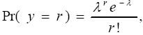
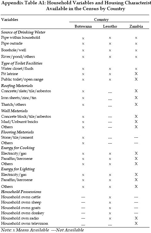
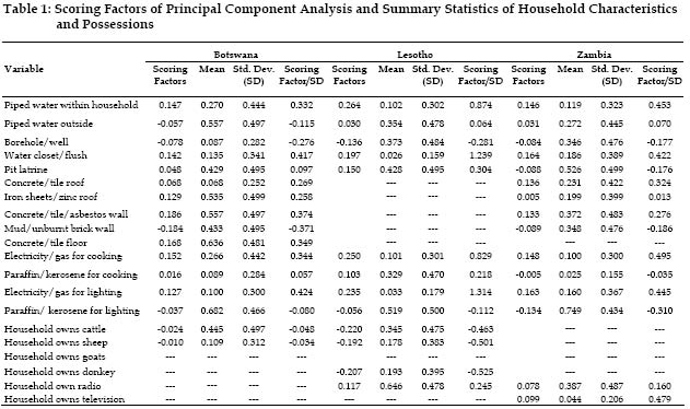
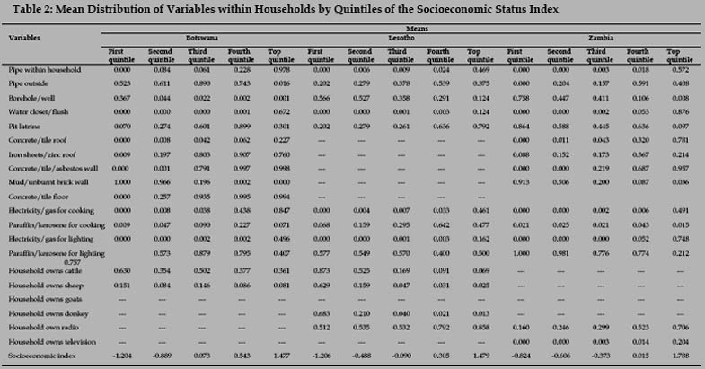
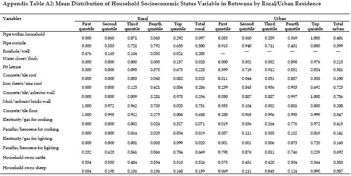
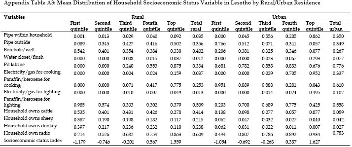
This means that y₁ and y₂ are linearly independent and the weight vectors (_1ii, a_2i, i=1, 2, 3…k) are constrained to sum up to one respectively. A third and higher number of components can be extracted as in y₁ and y₂ above until most of the variation is explained. After extracting the factor loadings, principal component analysis allows us to score these in order to create linear composites normalizing each variable (x) by its mean and standard deviation across households. Appendix Table A1 shows the variables used for the analyses by country. 

Table 1 below reports the scoring factors of the principal component analysis and summary statistics of the various variables. Each variable is dichotomous; therefore the mean and standard deviations range between 0 and 1. As can be observed in the first column under each country, there is a pattern in the factor scores. High positive scores are assigned to variables that are more likely to be associated with richer households and low or negative weights to those that are more likely to be associated with poorer households. For instance, positive values are assigned to pipe water within household, water closet/flush toilet, concrete or tile-walled households, households that use electricity or gas as either lighting or cooking energy, etc. On the other hand, low or negative values are assigned to households that have borehole/well as their source of drinking water, use a pit latrine, are built of mud or unburnt bricks, use paraffin or kerosene as their source of cooking or lighting energy, etc.

Since all variables are dichotomous, if we divide the scoring factors by the corresponding standard deviations, we can interpret the resulting coefficient for each variable as the contribution of that variable to the household’s assets or socioeconomic status index. Therefore, households that have pipe-borne water on their premises are higher on the socioeconomic status index by 0.33 inBotswana, 0.87 inLesotho, and 0.45 inZambia, than households that do not have pipe-borne water on their premises. Similarly, households that have water closet or flush toilet are higher on the index by 0.42 inBotswana, 1.24 inLesotho, and 0.42 inZambia than those households that do not use water closet or flush toilet. On the other hand, households that draw their drinking water from either borehole or well are lower on the socioeconomic status index by 0.28 inBotswana, 0.28 inLesotho, and 0.18 inZambia than households with piped drinking water. In all three countries animal possessions do not contribute positively to the socioeconomic status of households. This is surprising because in many rural areas of Africa wealth is stored in domestic animals.

Sorting households on the basis of their scores on the various indexes, we divided individuals within the households into quintiles ranging from the lowest 20% (first quintile) through the topmost 20% (last quintile) and summarized the mean distributions of the variables according to this classification presented in Table 2. If the index significantly mimics household socioeconomic status, we expect to see households in the topmost 20% having the highest mean values for those variables that scored higher on the index and this distribution should progressively decrease as one moves from the topmost to the lowest 20%. The results presented in Table 2 are consistent with expectation. For example, while 98% of the households in the highest 20% of the population have piped water on their premises in Botswana, none of the households in the lowest 20% have piped water on their premises. A similar pattern obtains for both Lesotho and Zambia for the same item—47 and 57% respectively for those in the topmost 20% as opposed to none in the lowest 20%. Similar distribution patterns are also observed for such items such as flush toilet, radio, and television. For example, while 71 and 20% of households in Zambia in the topmost 20% of the population own radio and television respectively, only 16% own radios and none own a television in the lowest 20% of the households.

Overall, the average socioeconomic status index ranges from –1.20 units among the lowest 20% of the households to 1.48 units among the topmost 20% in Botswana, –1.21 in the lowest 20% in Lesotho to 1.48 in the topmost 20% in Lesotho, and from -0.82 in the lowest 20% in Zambia to 1.79 units in the topmost 20%. The average difference in units of the index between the poorest 20% and the richest 20% of the population is 2.75 for Botswana, 2.69 for Lesotho, and 2.61 for Zambia. It is important to note that the definition of poverty does not follow the usual definitions, but is based on the factor scores obtained from the principal component analysis.

Recognizing the considerable differences between rural and urban areas in terms of the distribution of most of these items (variables) in many countries of Africa, we considered separately the analyses for rural and urban areas. Although the factor loadings and scores follow similar patterns for both the rural and urban areas as the overall for all three countries (not reported), the mean distributions show large differences between rural and urban areas by the different categories of the household socioeconomic index reported in Appendix Tables A2 and A3. For example, while just about 1% of the households in rural areas in Zambia have a water closet toilet on their premises, more than 43% of the households in the urban areas have a water closet toilet within the household. Similarly, while fewer than 1% of households in rural areas possess a television, more than 10% of households in urban areas possess one. The distribution of these items is even more skewed among the different socioeconomic status groups in the rural areas.

It might be argued that the socioeconomic status index may be influenced by community variables such as electricity or water supply, and therefore these variables should not be included in creating the index, since the ability of individuals within households to use these facilities may be constrained if such services are not available at the community level. While this argument might be plausible, it is important to note that housing characteristics not related to these community-level variables, such as type of construction materials, also show clear differences in terms of both the factor scores and their mean distributions among the different “poverty” groups of the index just as such community variables do, suggesting that these variables indeed reflect socioeconomic status within households. Furthermore, we argue that if such facilities are not extended to the community, both the poor and the rich alike may be constrained. On the other hand, we still find some households using such facilities in spite of the fact that they have not been extended to those communities, which suggests that these households are relatively wealthy ones since they may be using stand-alone generating plants to generate energy both for lighting and pumping water for domestic use.

An Application to Child Mortality

Returning to our theoretical model, we can argue that the level of childhood mortality is a reflection of the level of poverty in a society. We hypothesize, therefore, that mortality in childhood is likely to be higher among children in households considered poor than those in richer or higher socioeconomic status households. To ascertain whether this relationship is consistent with groups of the socioeconomic status index, we applied the index in a regression model estimating the likelihood of childhood mortality. If indeed the index does reflect socioeconomic status, childhood mortality is likely to be higher among households in the lower spectrum of the socioeconomic status groups than those in the higher spectrum. In separate models, we controlled for basic characteristics of women such as age and education and other factors such as household size, occupation of the head of household, and place of residence.

The method employed is based on event count data—the negative binomial regression model. This model is appropriate because the event of interest (child mortality) is based on a count of the number of children who have died among those ever born to women in households. The negative binomial model is based on a Poisson distribution that takes into consideration unobserved heterogeneity (Agresti, 1990; Long 1997; Allison, 1999; Hamilton, 2003). Assuming that y is a variable that can only have a nonnegative integer, then the probability that y is equal to r is given by:

where r=0,1,2….n; λ is the expected value of y; and r! is equal to r (r–1) (r–2)…(1).  The parameter λ depends on a set of explanatory variables, which can be specified in a simple Poisson model as:

Taking the log of λ requires that its value is not less than 0 for any of the x’s or β’s. A major property of the Poisson model is that for any given set of values on the explanatory variables, the variance of the dependent variable is equal to its mean (E(y) = var(y))

In practice, however, this is often not the case. The variance usually tends to be greater than the mean. Besides, the Poisson regression model does not take into consideration the effects of unobserved heterogeneity so that the combined effect of these problems often causes another problem called overdispersion. The problem of overdispersion leads to an underestimate of the standard errors thereby inflating the test statistics making the estimates inefficient (although they may be consistent) (Long 1997). This problem can be corrected using the negative binomial model, which incorporates an error term in the model to account for unobserved heterogeneity specified as:

The assumption here is that the dependant variable y_i has a Poisson distribution with expected value λ_i conditional on ε_i, ε_i having a standard gamma distribution (Agresti, 1990; Long, 1997; Allison, 1999). The idea for the inclusion of ε_i is that this captures the effects of unobserved variables excluded from the model. To adjust for exposure, another term (log(τ)) is included as an offset, whose coefficient is constrained to 1. The variable used as an offset in this paper is children ever born (CEB), which aims to account for the effect of fertility and duration of exposure. The dependant variable is a count of the children dead. 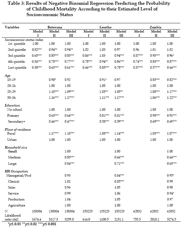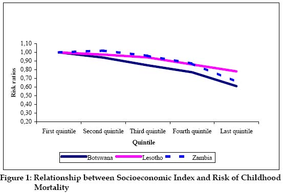The model is estimated using maximum likelihood procedures.

RESULTS

For each country we ran three separate models using children dead as the dependant variable, with the socioeconomic status index as the main predictor variable of interest. Model I for each country considered only the gross effect of the index on the chances of child survival or mortality at the household level and models II and III controlled for the age and education of the mother and the size of the household and the household head’s education respectively. The results are reported in Table 3. 

Examining the gross effect of the association between the socioeconomic status index and childhood survival, results of the negative binomial regression show that the probability of dying in childhood decreases from the poorest (first quintile) 20% of the population to the richest (last quintile) 20%. For instance, comparing the chances of childhood mortality in Botswana between the poorest 20% of the population and the rest of the groups, it is observed that the risk of childhood mortality is reduced by about 18% in the second quintile (second poorest) and further down to about 62% in the last quintile (richest 20%) compared with poorest. Similar patterns are observed for both Lesotho and Zambia respectively, although the effect in those two countries is not as dramatic as in the case of Botswana.

The pattern persists even when we control for other factors (models II and III). It appears, however, that there is not much difference between the first two socioeconomic status groups (i.e., those in the first and second 20% of the population) in both Lesotho and Zambia because the chances of childhood mortality are about the same for both groups in the two countries. Although it is not possible to compare across countries directly, it seems there is more disparity or inequality among the groups in Botswana than in either Lesotho or the Zambia, a conclusion that can also be drawn from the average difference in units of the index between the poorest 20% and the richest 20% of the population in the three countries discussed earlier.

In Figure 1, we display the mortality rate ratios (risk ratios) by the socioeconomic status index for the three countries. Note that the graphs present results of the third model for each country, thus showing the net effect of the socioeconomic status index since the third model in each case controls for the other factors—the age and education of mothers, household size, occupation of the head of household, and rural/urban residence. Clearly, the graph shows a negative relationship between child mortality and socioeconomic status or poverty. The chances of childhood mortality are lower at higher levels of socioeconomic status than at lower levels of the index.   

With regard to the effect of the other variables, they all show the expected relationships, except for age where children of mothers in age groups 15–19 appear to have lower chances of mortality compared to the other age groups. This is surprising because children of women in this age category would seem to be at a higher risk of mortality than their counterparts with older mothers, since the majority of women in the 15-19-year age category may be first parity women and may not be as experienced in child care as their older counterparts. Apart from inexperience, their pelvises may not be as well developed such that their children are more likely to be at higher risk of birth injury and other related risks including malformation. The finding that these children have lower mortality risks may be due to poor data; Preston and Haines (1991) noted that results from women in this age group tend to be “erratic.” With regards to household size, the results suggest that the chances of child mortality are lower for medium and larger households than for children in smaller households, a result that is contrary to the views of the pro-Malthusian school, which argues that larger numbers of people constrain resources, which may have an adverse effect on survival. Nonetheless, the result makes sense because, all things being equal, households where children die will decrease in size compared to those where children survive. A household is classified as small if 5 or fewer people reside in it, medium if between 6 and 10 people reside in it, and large if more than 10 people reside in it. It should be noted, however, that the relationship does not appear to be linear, as the risk ratio is slightly higher in the large households than in medium households with reference to the smaller households. It appears that the head of household’s occupation does not seem to matter much except for those in managerial/professional positions. On the other hand, the effect of education as expected is very strong and in the expected direction; i.e., the chances of childhood mortality decline significantly as the mother’s education increases. This relationship is pervasive and strong in all three countries.

SUMMARY& CONCLUSIONS

Lack of income and other direct indicators of poverty and socioeconomic status in Africa have often restricted the capacity of researchers to explore the relationship between poverty or social status and different demographic phenomena of interest. On the other hand, it is possible in many countries of Africa, and indeed, elsewhere in other parts of the developing world, to differentiate households simply by the type of consumer durables and other possessions they own and by the type of construction materials the households are made of.

To ascertain whether these variables do indeed differentiate households on the basis of their socioeconomic status, which normally is indexed by income, we created an index of household socioeconomic status and categorized the population into five social status or poverty groups and then explored the relationship between these groups and childhood mortality. The results are reassuringly consistent with expectation, both simply by examining the mean distribution of the different variables according to the socioeconomic groups and also by their relationship to childhood mortality in a multivariate regression model. The chances of childhood mortality decrease consistently with high levels of the socioeconomic status index.

This analysis suggests the possibility of employing information on household characteristics and possessions often gathered in African censuses to do demographic analysis, especially in situations where the interest of researchers relates to household socioeconomic differences but are constrained because of lack of income data or other direct measures of economic status. Indeed, given the fact that income data are normally either poorly reported or deliberately misreported in most settings, it appears that these measures present a more credible means of differentiating population groups in terms of their socioeconomic status than income data in many developing countries.

One major concern that may be raised, especially related to use of the composite index to correlate mortality, is the question of how to determine the differential contribution of the individual variables used in creating the index since some of these variables may have direct and independent effects on childhood mortality. In response to this concern, it must be borne in mind how we conceptualize the index. If the index is conceptualized as representing the combined effect of these variables on mortality, then this concern is indeed valid. On the other hand, if we conceptualize the index as a proxy for income, as in this particular case, then there is no need to worry about the individual effects of the various variables. Another concern that has often been expressed relates to the fact that the availability of variables like electricity and water supply in households is partly determined by their availability in the community. While this may be a concern, as we noted elsewhere in the paper this problem relates to both the poor and the rich alike and so we do not expect this to bias the index in any way.

REFERENCES

• Agresti, A. 1990. Categorical Data Analysis. New York: John Wiley.

• Allison, P. 1999. Logistic Regression Using the SAS System: Theory and Application. Cary, NC: publisher?

• Ayad, M., B. Barrère, and J. Otto. 1997. Demographic and Socioeconomic Characteristics of

• Households. Demographic and Health Surveys, DHS Comparative Studies No. 26, Calverton, MD: Macro International.

• Cleland, J.G. and J. K. van Ginneken. 1988. “Maternal Education and Child Survival in Developing Countries: The Search for Pathways of Influence,” Social Science and Medicine 27 (12):1357–1368

• Duncan, O.D. 1984. Notes on Social Measurement: Historical & Critical, New York:Russell Sage  Foundation.

• Dunteman, G.H. 1989. Principal Component Analysis, Quantitative Applications in the Social Sciences, No. 69 PUBLISHER?

• Filmer, D and L. Pritchett. 2001. “Estimating Wealth Effects without Expenditure Data – or Tears: An Application to Educational enrollments in the States of India,”  Demography 38(1): 115–132

• Hamilton, Lawrence C. 2003. Statistics with STATA: Updated for Version 7. Duxbury Thomas Learning. LOCATION?

• Hobcraft, J.N., J.W. McDonald, and S.O. Rutstein. 1984. “Socio-economic Factors in Infant and Child Mortality: A Cross National Comparison.” Population Studies 38: 193-223

• Long, J.S. 1997. Regression Models for Categorical and Limited Dependent Variables Advanced Techniques in the Social Science Series. Location: Sage Publications.

• Mazumdar, K. 1999. “Measuring the Well-being of the Developing Countries: Achievement and Improvement  indices,” Social Indicators Research 47: 1-60.

• McKweon, T. 1976. The Rise of Modern Population. New York: Academic Press.

• Mckweon, T. and R.G. Record .1962. “Reasons for the Decline of Mortality in England and Wales during the nineteen Century,” Population Studies 16 (2): 94-122.

• McKweon, T, R.G. Record, and R.D. Turner. 1975. “An Interpretation of the Decline of Mortality in England and Wales during the Twentieth Century,” Population Studies 29(2): 391-422.

• Montgomery, M.R., M. Gragnolati, K.A. Burke, and E. Paredes. 2000. “Measuring Living Standards with Proxy Variables,” Demography, 37: 155-174.

• Mosley, W.H. and L.C. Chen. 1984. “Analytical Framework for The Study of Child Survival in Developing Countries,” in W.H. Mosley and L.C. Chen (eds.), Child Survival: Strategies for Research, Population and Development Review, a Supplement to vol. 10.

• Muhuri, P.K. 1996. “Estimating Seasonality Effects on Child Mortality in Matlab,  Bangladesh,” Demography 33: 98-110.

• Preston, S.H and M.R. Haines. 1991. “Child Mortality in Late Nineteenth-Century America,” in Editor? Fatal Years. Princeton, NJ: PrincetonUniversity Press, PP?

• Sastry, N. 1996. “Community Characteristics, Individual and Household Attributes, and Child Survival in Brazil,” Demography 28: 211-229.

• Sen, A. K. 1985. Commodities and Capabilities. Amsterdam: North-Holland.

• ___. 1987. The Standard of Living. Cambridge: CambridgeUniversity Press.

• ___.  1999. Development as Freedom. New York: Publisher?

• ___. 1992. Inequality Re-examined. Boston: HarvardUniversity Press.

• Tabutin, D and E. Akoto. 1992. “Socio-economic and Cultural Differentials in the Mortality of Sub-Saharan Africa,” in Mortality and Society in sub-Saharan Africa, E. van de Walle, G. Pison, and M. Salad-Diakanda (eds.). Oxford: Clarendon Press, pp. 32–64.

• Todaro, M.P. 1978. Economic Development in the Third World. LondonL: Longmann.

• United Nations. 1985. Socioeconomic Differentials in Child Mortality in Developing Countries, ST/ESA/SER. A/97. New York.

• UNDP. 1990. Human Development Report 1990, Oxford:  OxfordUniversity Press.