 |
| About Bioline | All Journals | Testimonials | Membership | News |
|
||||||
|
||||||
African Population Studies/Etude de la Population Africaine, Vol. 20, No. 1, 2005, pp. 1-17 Using WinBUGS to Study Family Frailty in Child Mortality, with an Application to Child Survival in Ivory Coast Marie-Claire Koissi, Göran Högnäs Department of
Mathematics, Åbo Akademi
University, Fanriksgatan
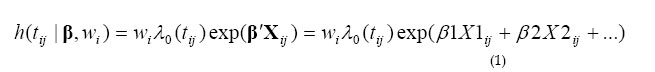
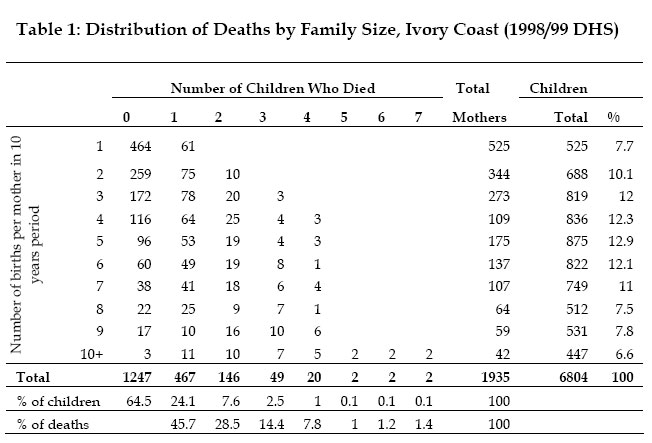
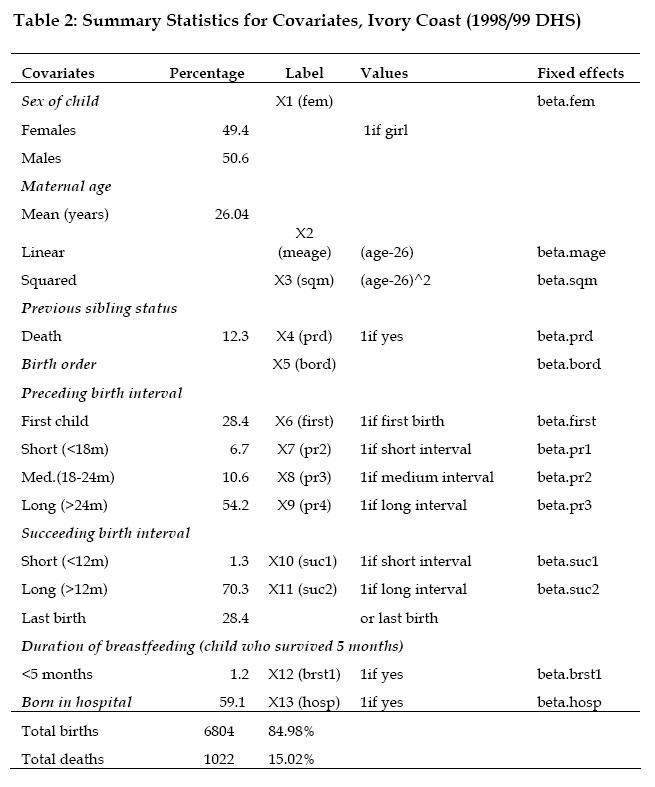
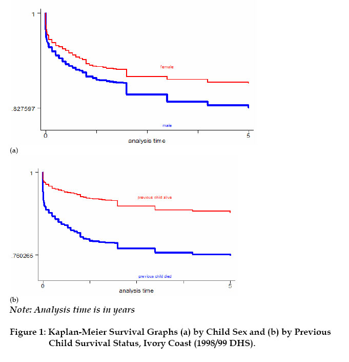
3B, 20500 Turku, Finland Code Number: ep05001 Abstract This article analyzes the effects of unobserved family heterogeneity in children survival times through a Bayesian approach. We rely on survey data from Ivory Coast and use a proportional hazard model with multiplicative random effect. With such a model, the usual assumption of independence of observations is avoided. The posterior distributions of the parameters are estimated through a Gibbs sampler algorithm using the WinBUGS software. This technique overcomes the possible local convergence problem observed with the commonly used Expectation-Maximization method. Introduction Under-five mortality rate for the world dropped from 193 per thousand births in 1960 to 86 in 1998, which corresponds to 55 percent decrease (UNICEF, 2001). In Sub-Saharan Africa, the reduction in mortality rates for children aged 5 and younger, between 1960 and 1998, was nearly 34 percent (from 261 to 173 per thousand births). For example, in Ivory Coast, the same source indicates that under-five mortality rate decreased from 300 to 150 per thousand births between 1960 and 1998. Although much progress has been made in terms of prevention and child care, under-five mortality rates in the Sub-Saharan African region remain high, compared to the mortality rate of 6 per thousands births observed in the industrialized countries in 1998 (UNICEF, 2001). A number of studies have focused on the factors affecting children mortality (Manda, 1999; Kuate-Defo, 1992; Akoto and Tabutin, 1990; Pebley and Stupp, 1987; Martin et al., 1983, among others). These researches showed that child mortality in developing countries was mainly associated with measurable socio-economic conditions such as nutritional status and poor living conditions. However, some unmeasured genetic, environmental and behavioural components still remain non-negligible. In effect, children belonging to the same family share certain unobserved characteristics (or heterogeneity), which may not be sufficiently described by the covariates included in the earlier standard models (Guo and Rodriguez, 1992). The ignorance of such family-level correlation may lead to biased parameters estimates. This unobserved heterogeneity, also referred to as frailty (Vaupel et al., 1979), operates at three different levels, at least: child, family and community (Sastry 1997). At the family level, children from the same parents inherit common genetic factors and usually grow up in the same household environment. Parents are also more likely to adopt similar child care behaviour for all their children. Genetic factors remain the major component of the family-level frailty. However, each child has a proper susceptibility to infection, independently of his family membership (Childs et al., 1992). This idiosyncratic genetic factor remains the major child-level unobserved frailty component. In addition, inside the common global family behavioural factor, parents may adopt a slightly different prenatal and neonatal attitude from one child to the next: the length of the breastfeeding period, the health care practice and the nutritional status, for example. At the community level, the random effects are more likely of behavioural and environmental nature. During the last ten years, the unobserved heterogeneity has been intensively associated to child mortality studies: Guo and Rodriguez (1992) and Guo (1993) applied a multivariate proportional hazard model to capture the family-specific random effects on clustered data from Guatemala; a logistic model with family random effects was used to examine the frailty common to all children from same mothers in Brazil (Curtis et al., 1993) and Bangladesh (Zenger 1993); Ronsmans (1995) investigated the patterns of family-level clustering in a rural community of Senegal; Sastry (1997) also presented a hazard model with nested frailty to control for unobserved family and community effects in data from Brazil. More recently, Kuate-Defo (2001) estimated a model for hierarchically clustered data and applied it to child survival in Cameroon. The models' parameters and the distribution for the random effects were generally estimated via the Expectation-Maximization (EM) algorithm (Manda, 2001; Sastry, 1997; Curtis et al., 1993; Guo and Rodriguez, 1992). The EM algorithm is an iterative method, which heavily relies on the choice of starting values. Hence, it may converge toward a local maximum instead of the global one (Sinha and Dey, 1997). To circumvent this problem, a full Bayesian approach, which uses Markov Chain Monte Carlo methods, can be used. Recently, Bayesian frailty models have been developed successfully for child survival data in Mali (Gemperli et al., 2004), Minnesota (Banerfee et al., 2003) and Malawi (Bolstad and Manda, 2001). Kandala et al. (2002) also used Bayesian approach to analyse the determinants of undernutrition in Malawi, Tanzania and Zambia. Unlike the EM algorithm, the Bayesian approach avoids the computation of cumbersome high-dimensional integrals (Manda, 2001). The goal of this work is to investigate family heterogeneity in child mortality data from Ivory Coast, from a Bayesian perspective. The analysis is based on a proportional hazard model with multiplicative random effects. In that case, the independence between observations from the same family, which is a slightly restrictive assumption, is not required. The contribution of the present work is implementing Bayesian multiplicative frailty model on WinBUGS, which would be useful to practitioners. The remainder of the paper is organized as follows. In Section 2, the data and the covariates of interest are described. The Bayesian model and the computation approach are presented in Section 3. The results are given in section 4 and a comparison with standard analysis is also discussed. Section 5 contains some concluding remarks. Data and Covariates Data A representative sample of 3,040 women, aged 15-49 years, result from the Demographic and Health Survey (DHS, 2001) carried out from September 1998 to March 1999 inIvory Coast. The survey questionnaire included a complete birth history, as well as information on maternal education, household and related subjects. A total of 6,804 births by 1,935 women were single (non-twin). This sample constitutes the study data in which 1,022 children (i.e. 15 percent) died by the time of the interview. Table 1 shows the distribution of children by family. The 1,935 mothers having non-twin births represent the family subdivision. The number of births per mother varies between 1 and 14 with a mean of 3.52. A non-negligible level of family random effect is expected, since more than 90 percent of the children belong to families that contribute two or more births (Sastry, 1997). Community or district stratifications might be worth exploring in future work, using WinBUGS. Covariates The covariates used in this study consist of the mother’s age (at birth of child), the child's age and sex, the child's birth order, the preceding and succeeding birth intervals, the survival status of the previous child, the duration of breastfeeding and whether birth occurred in hospital (referred here to all medical centres, public or private) or not. Information (taken at the time of interview) on household income, father/mother's occupation and education level had been omitted because they might have changed during the time preceding the interview. Neither was the mother’s marital status used. For the same reason, the household variables such as the source of drinking water and the place of residence are not included in the model. It is worthwhile that future work should consider the effects of these important time-varying covariates. Maternal age (at birth of the child) is a commonly used covariate. Previous studies showed that children born from women at youngest and oldest age are generally subject to highest risk of death (Sastry, 1997; Pebley and Stupp, 1987; Trussell and Hammerslough, 1983). However, Martin et al. (1983) found that children born from oldest women have a lower mortality risk in data from Indonesia and Pakistan. Lalou and Legrand (1997) found the same puzzling effect of mother's age on child mortality in Bamako, Mali. Child mortality risk also differs by sex of the child: mortality is higher among boys than girls, at least during the first months of life (Waldron, 1987; Trussell and Hammerslough, 1983). Large birth order is generally risky for child survival. But first born children also experience a high mortality rate (Hobcraft et al., 1985). Findings from several studies suggest that short preceding and succeeding birth intervals largely increase child mortality risk (Guo, 1993; Miller et al., 1992; Pebley and Stupp, 1987). However, Koenig et al. (1990) found a lower effect of short birth spacing. Breastfeeding duration also affects child mortality risk (Manda, 1999). Short breastfeeding duration is generally associated with higher child risk of death (Cantrelle and Leridon, 1971). Table 2 gives the summary statistics of the variables used in the study. There is as many boys as girls in this sample. The table also indicates that the mean maternal age is 26 years. About 12 percent of the children have experienced the death of previous sibling. More than 50 percent of the preceding and succeeding birth intervals are long. The table also shows that mothers generally give birth in medical centre (called “maternité”) and most children are breastfed, at least during the first five months following birth. Non-parametric analysis of the children survival times are obtained using the Kaplan-Meier (KM) survival curves (Kaplan and Meier, 1958). Figure 1 shows the KM survival curves by child’s sex and by survival status of previous sibling. Male children have higher risk of death, as well as children whose previous sibling died by index's child birth. The graphs (not displayed here) also show that children with longer preceding/succeeding birth interval have greater survival chance. The Bayesian Model Denote by tij the random survival time of the j th child from family i and θ =(β, wi )the unknown parameters of the model corresponding to the data. The parameter wi represents the family random effect and β = (β1,β 2,..)is the vector of fixed effect coefficients. The family random effect is assumed to act on the conditional hazard h( tij |β ,wi) in the following multiplicative way:
Our aim is to find the distribution of the family unobserved heterogeneity wi. The classical likelihood-based method assumes that the unknown model parameters have true fixed values, which are found by optimization. The Bayesian approach, however, updates the prior belief (π( β ,wi )) using the data, in order to obtain the posterior distribution (which represents new beliefs after having observed the data). The posterior distribution of ( β ,wi ) conditioned on the data is proportional to the product of the likelihood function and the prior distribution (Gelman et al., 1995)
Let us introducethe censoring indicator δij such that δij equal 1 if the child has died and 0 if not. If fijand Sijare the density and the survival functions respectively, then the following equality holds: The contribution of child j from family i to the likelihood function isits density function if the child dies, and its survival function otherwise:
where Previous studies have shown that the effect of the chosen covariates on child mortality do not have equal importance over the whole period of childhood (Sastry, 1997; Guo and Rodriguez, 1992). Therefore, a piecewise exponential baseline hazard can be used. In particular, based on preliminary analysis not shown here, the study time period was split into five intervals with cut points at 2.4, 6, 12 and 24 months. Within each interval In the baseline hazard is assumed constant: λ(tij)= λn for tij ε In . Under that assumption, the likelihood function coincides with that of a Poisson distribution with mean Eijn λijn (Laird and Olivier, 1981 [11]). In that expression, Eijn denotes the time lived in the interval In by the jth child from the ithfamily and the parameter λijn is the corresponding hazard function. The Prior SpecificationThe choice of the prior distributions follows from previous studies (Gemperli et al., 2004; Bolstad and Manda, 2001). To compute the prior distribution, π( β ,wi ), the matrix of fixed effects β is set to follow a multivariate normal distribution with zero mean and low precision: β ~Nq (O,Σ) , where Σ is a diagonal covariance matrix with large variance terms. The integer q is the total number of covariate terms in the model. Hence, the joint density function of β is
A widely use conjugate prior is adopted for the family frailty :wi~ Gamma(τ ,τ ). The hyper-parameter τ is also assumed Gamma distributed. The Full Model A proportional simplification of the posterior density is obtained from (2): 
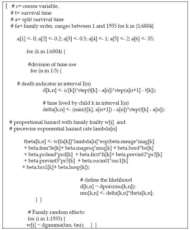
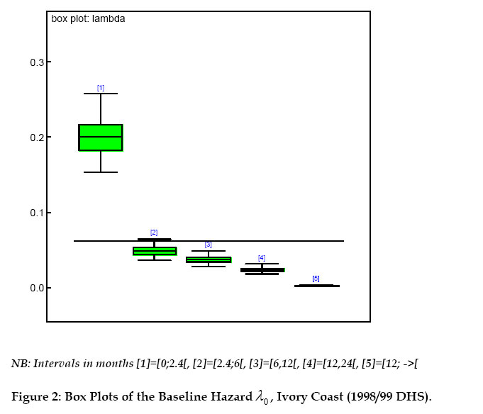
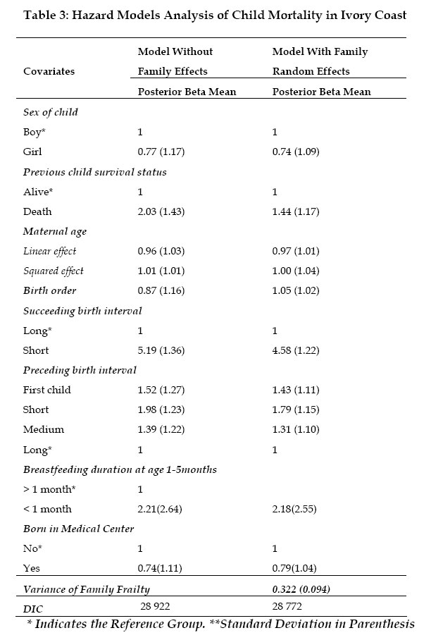
Since that posterior distribution is analytically as well as numerically hard to obtain, a Markov Chain Monte Carlo (MCMC) simulation is performed. The idea is that, if a specific Markov chain is run (after a suitable initial burn-in period) for long enough time, it should reach a stationary distribution which is the same as the desired posterior distribution (Gelman et al., 1995).Following previous studies on hierarchical model (Gelman et al., 1995), the distributions of the nodes, conditional on all the parameters, are assumed independent of each other. In addition, the prior distributions of any fixed/random effects are independent. The Computation A Gibbs sampling, as implemented in the WinBUGS (Spiegelhalter et al., 2003) software, is used to sample from the posterior density of the family random effect wi. However, one could also write a Fortran code, as previously done by Bolstad and Manda (2001), which requires longer time for coding and testing. WinBUGS saves the researcher from these complexities, and thus, allows him to concentrate on more substantive issues. An outline of the WinBUGS code written by the authors is displayed in Appendix 1. The WinBUGS step function in the code is such that step(x) = 1 if x ≥ 0 and 0 otherwise. The data organization is also a key requirement: since the data are mostly unbalanced, a rectangular format may lead to wrong estimates. Hence, a nested indexing format must be preferred. Four chains with different starting values were run simultaneously. After 2000 iterations for burn-in, 5.000 iterations were performed for each chain and one out of every 100th values were used. The obtained time series alone are not sufficient criterion to conclude that the chains converge. Therefore, the Gelman-Rubin factors (Gelman and Rubin, 1992) were also examined. This factor compares the variation in the sampled parameter values within and between chains (Congdon, 2003). Thus it describes how much the increase in the number of iterations may improve the estimates. Values under 1.2 correspond to approximate convergence of the Markov chain. WinBUGS produces scale reduction factors that are very close to 1 for the fixed effects. For the family frailty and its variance, the obtained Gelman-Rubin factor ranged between 0.7 and 1.3 for the first thousand iterations. Then, values around 1 were obtained after 2500 iterations. These results do not contradict the convergence observed from the historical time series of the chains. Results Figure 2 presents the values of the baseline hazard → by time interval. The observation period was split into the following five intervals (in months): [0, 2.4), [2.4,6), [6,12), [12,24) and [24,à ). Similarly to previous studies (Guo and Rodriguez 1992, Sastry 1997, Bolstad and Manda 2001) the mortality risk is higher in the first two months of life and then, it continuously decreases. The high risk of death at young age may be due to inadequate delivery conditions and lack of prenatal vaccination in order to guarantee child immunity against childhood diseases. Household characteristics (nutrition and hygiene) may also contribute to high mortality risk at lower age. We estimated
two models: Model I uses the covariates previously defined, without any family
frailty term. Model II includes the same covariates as in Model I and allows
for clustering by family. Table 3 depicts the relative effects obtained for
both models. The relative risk for each covariate is obtained by taking the
exponential of its beta value (given as WinBUGS output). The deviance
information criterion (DIC), as defined by Spiegelhalter et al. (2002),
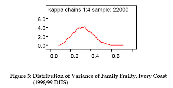
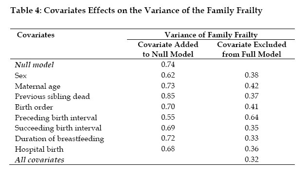
is used for models comparison: For Model I, the table indicates that mortality risk is slightly higher among boys than girls, as shown in some previous studies (Trussell and Hammerslough 1983, Bolstad and Manda 2001). The relative risk of death for girl is 0.77 times the risk for boys. However, that sex effect is not statistically significant (Pebley and Stupp, 1987). The results also show that children whose previous sibling died experienced a lower survival chance. When the reference group has a preceding birth interval greater than 24 months, a preceding birth interval less than 18 months increases the child mortality risk (about 2 times). Similarly, when the group with succeeding birth interval greater than 12 months is taken as the reference, the relative risk of death, among children with shorter succeeding birth interval, is five times higher. First births are also 1.5 times riskier. Relative risks of 0.96 and 1.01 are obtained for maternal age linear and squared effect respectively. Additional computations suggest a positive correlation (ρ =0.7) between maternal age squared and death of previous child. Birth order is strongly negative correlated to maternal age squared (ρ = -0.8) as well as to linear maternal age (ρ =0.7). Last column of Table 3 depicts the results of Model II, which includes multiplicative family frailty. Compared to Model I, the mortality risk associated with child sex remains unchanged, as well as the risk related to maternal age, succeeding and preceding birth intervals, breastfeeding duration and hospital birth. However, a remarkable difference is that the relative effect of the birth order slightly increased (from 0.87 to 1) by including the family frailty term. Moreover, the posterior mean for the survival status of the previous child is lower in the model with frailty: a relative effect of 2.03 against 1.44 (when the model incorporates family frailty). Similar result was found by Sastry (1997) in Brazil and Guo (1993) in Guatemala. This suggests that in the model with family frailty, the risk related to the previous child death has been captured by the family effect (Bolstad and Manda, 2001). The deviance information criterion values suggest that Model II, which includes the family frailty, produces the best fit. The posterior distribution of the family frailty is shown in Figure 3. A posterior mean of 0.322 is obtained for the variance of the frailty, after controlling for the variables defined in Table 2. This result means that, the death of one child in a family increases the risk of death of the index child by about 32% (Guo, 1993). Guo and Rodriguez (1992) found a variance of 0.22 for family random effect in Guatemala, Sastry (1997) obtained 0.516 for Northeast Brazil and Bolstad and Manda (2001) reported a variance of 0.843 for Malawi. The sensitivity of the family frailty effect to the different models is also explored. This is done by studying the variance of the family frailty when, first, each covariate is added to an initial null model with child age only. Secondly, we report how the variance of the frailty changes, when each covariate is removed from a full model (which includes all the covariates). Table 4 shows the outcomes of this analysis. These results suggest that the explained family random effect is mostly represented by the preceding birth interval. Sastry (1997) found similar predominance of the preceding birth interval. Concluding Remarks We used a Bayesian approach, implemented in WinBUGS, to explore the effects of family membership on child mortality risk. A proportional hazard model with multiplicative family frailty was applied to data from Ivory Coast 1998/99 Demographic and Health Survey. The analysis shows that the covariates related to birth spacing (short succeeding/preceding birth intervals) are high risk factors. In fact, reduced birth spacing leads to large family size, which affects mother's health condition during each pregnancy. As a consequence, the children have high risk of death due to small weight at delivery, competition between siblings for nutritional and affective resources or high risk of transmission of infectious diseases among siblings (Ronsmans, 1995). That result confirms the conclusion of previous works: a great attention should be given to teaching family planning to women. This is not widely applied even when its benefits are known. That study also supports the view that the death of previous child increases the indexed child mortality risk. The premature death of a child may expose the non-breastfeeding mother to the risk of new pregnancy, while her body is still physically (and mentally) weak. Thus, the future children may not be healthy at delivery, due to improper foetal development (Scrimshaw, 1996). Important family random effect was also found (with a variance of 0.32). WinBUGS models hierarchical child mortality data, without requiring cumbersome computation of integral (unlike the Expectation-Maximization algorithm). This method offers various extensions worth studying: infant mortality model with spatial (community) structure needs to be implemented in WinBUGS. Hence, graphical representation of regions with high mortality rate could be conducted, which would help define targeted policies. Acknowledgement The authors would like to thank the Demographic and Health Surveys program (www.measuredhs.com) initiated by the U.S. Agency for International Development (USAID) for providing the corrected data. Financial support from Magnus Ehrnrooth foundation and the Academy of Finland, project no. 200891, is gratefully acknowledged. We are also greatly indebted to two anonymous reviewers for their constructive comments on the earlier version of the paper. References
Appendix 1: Outline of the Code written in WinBUGS Copyright 2005 - Union for African Population Studies |

