Journal of Applied Sciences & Environmental Management, Vol. 9, No. 1, 2005, pp. 51-55

New Solutions of Stokes Problem for an Oscillating plate using Laplace Transform

¹EHSAN ELLAHI ASHRAF; ²MUHAMMAD R. MOHYUDDIN

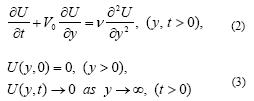
¹College of Aeronautical EngineeringNationalUniversity of Sciences & Technology PAF Academy24090, Risalpur, Pakistan
²Department of Mathematics Quaid-i-Azam University45320, Islamabad, Pakistan

Code Number: ja05009

ABSTRACT:An exact solution of the flow of a Newtonian fluid on a porous plate is obtained when the plate at y = 0 is oscillating with the amplitude β and oscillating frequency ω with the assumption that the plate initially is at rest and that the velocity approaches zero as we go far from the boundary region. The fluid flow problem is solved with the help of Laplace transform technique. Here we discuss two cases: first case corresponds the oscillating porous plate with superimposed suction or blowing and second deals with an increasing or decreasing velocity amplitude of the oscillating flat plate. @JASEM

The Initial boundary value problem and the solution

 Let us assume that the x - coordinate is parallel to the porous flat plate and y - coordinate perpendicular to it and also that the fluid initially is at rest. For t > 0 the flat plate is moved periodically with the following velocity (Turbatu et al., 1998).

where ω is the oscillating frequency of the plate at y = 0. The initial value problem is given by (Schilichting, 1982)

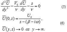
where V₀ < 0 is the suction velocity, V₀ < 0 is the blowing velocity, v = μ/p is the kinematic viscosity of the fluid and U (y,t) is the velocity of the fluid at a point.

The Laplace transform of U (y,t) is defined by

The transform problem takes the form

The solution of (5) subject to boundary conditions (6) is given by

              (7)

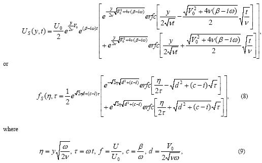
Finally, the Laplace inverse of (7) leads to the following form

 and erfc is the complimentary error function.

The solution (8) corresponds a small time solution. The real part of the velocity is given as

                (10)

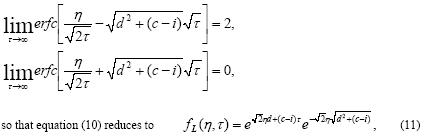
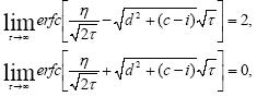
The solution (8) or (10) is for small times and describes the combined effect of suction/blowing and acceleration/deceleration for an oscillating plate. In order to find the solution for large times we proceed as:

For large time we take (η/2τ) << 1,τ >> 1 and            

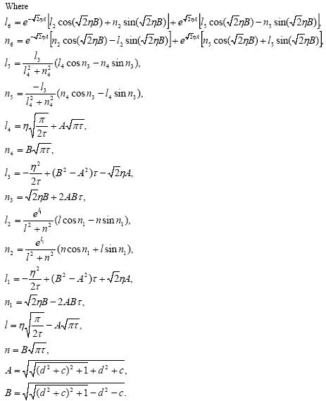
where f_L denotes the solution for large times. The real part of the solution (11) is given by

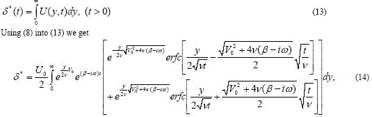
where A and B are defined in (10).

The displacement thickness, δ* (t), is defined as

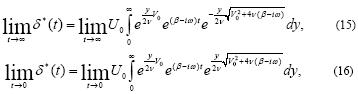
For V₀ = β = 0 we obtain the classical viscous case. In the limiting cases of and  we get the following

We see from (15) that when t →  the displacement thickness δ* (t), no matter whether it is the case of acceleration or deceleration. But from (16) we get

where must be negative, which means it will converge only for the suction case and not for the blowing case.

Special Cases

To understand the different physical aspects of the solution (10), we discuss some special cases.

Oscillating Plate

The results of Stoke’s second problem can be obtained far from the plate when τ → 

and by taking c = d = 0 in (8) i.e.

f _ST (η, τ) = exp ((1- i) η) exp (-iτ)      (13)

Oscillating Porous Plate c = 0, d 0

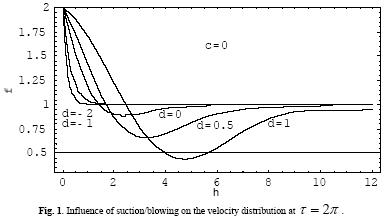
The solution for velocity component f is plotted in fig. 1. for a fixed time τ = 2π as a function of the suction/blowing velocity V₀, given by . The values d = 0 refers to the classical Stoke’s problem. It is noted that the boundary layer thickness is controlled by the suction velocity (V₀ < 0) i.e. In case of blowing (V₀ > 0), the boundary layer thickness becomes large as is expected physically.

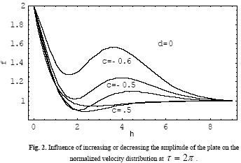
Oscillating plate with acceleration/deceleration d = 0, c 0  

In this section, the superposition of two time dependent functions is taken into account. One of which is due to the oscillation of the plate with imposed frequency ω and the second is an exponential increase or decrease of the velocity amplitude of the plate with the parameter β₀.

The parameter c =b₀/ω gives the variation of the amplitude of the plate velocity and c = 0, implies the classical viscous case. The solution (10) is plotted in Fig. 2. for τ = 2π and for different values of c =b₀/ω.