+Bioline International Official Site (site up-dated regularly)

Journal of Applied Sciences & Environmental Management, Vol. 9, No. 3, 2005, pp. 31-36

Controllability and Null Controllability of Linear Systems

^1*DAVIES, I; ²JACKREECE, P

¹Department of Mathematics and Computer Science, Rivers State University of Science and Technology, P.M.B 5080, Port Harcourt, Rivers State, Nigeria. Email: davsdone@ yahoo.com
²Department of Mathematics, Rivers State College of Education, Port Harcourt, Rivers State, Nigeria. Email: preboj@yahoo.com Mobile Phone: +234-803-673-0979

*Corresponding author: Email: davsdone@ yahoo.com

Code Number: ja05055

ABSTRACT:

This paper establishes sufficient conditions for the controllability and null controllability of linear systems. The aim is to use the variation of constant formula to deduce our controllability grammiam, by exploiting the properties of the grammiam and the asymptotic stability of the free system, we achieved our results. @JASEM

Differential equations, in general, are an important tool for harnessing into single system and analyzing the inter-relationship between different components which otherwise may continue to remain independent on each other. It is known in Sebakhy and Bayoumi (1973) that, in the study of economics, biology and physiological systems as well as electromagnetic systems composed of such subsystems interconnected by hydraulic, mechanical and various other linkages, one encounters phenomena which cannot be readily modeled unless relations involving time delays are admitted. Models for such systems can be controlled. A delayed control on such systems will affect the evolution of the system in an indirect manner (Artstein and Tadmore, 1982), where the decisions in the control function are shifted, twisted or combined before affecting the evolution. Models for systems with delay in the control occur in the study of gas-pressures bipropellant rocket systems, in population models and in some complex economic systems etc.

The controllability of systems with delays in the control has been studied by several authors see (Balachandran, 1987; Balachandran and Dauer, 1996; Chukwu, 1979; Onwuatu, 1989). In particular Manitius and Olbrot (1972) studied the system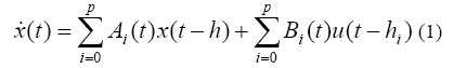

and gave sufficient conditions for the relative controllability of (1). Our interest, is to integrate the concept of null controllability into a generalized system with delay in state and control given by

We shall give sufficient conditions for the null controllability with constraint of (2) when relative controllability is assumed. Our results complement and extend known results.

BASIC NOTATIONS AND PRELIMINARIES

Let n and m be positive integers, E the real line (-∞, ∞). We denote by Eⁿ the space of real n- tupples with the Euclidean norm denoted by | · |. If J is any interval of E the usual Lebesgue space of square integrable (equivalent class of) functions from J to Eⁿ will be denoted by L₂(J, Eⁿ). L₁([t₀ ,t₁], Eⁿ).denotes the space of integrable functions from [t₀ ,t₁] to Eⁿ . Let h > 0 be given, for functions x:[t₀ - h ,t₁]→ Eⁿ, t ε [t₀ ,t₁], we use x_tto denote the functions on [-h,0] defined by x_t(s) = x(t + s) for s ε [-h,0]

Consider the system

Embed (3)

where

EMBED (4)

satisfied almost everywhere on [t₀ ,t₁]. The integral is in the Lebesgue- Stieltjes sense with respect to s. L .(t,Ø) is continuous in t, linear in Ø. η (t.s) is an n x n matrix function measurable in t and of bounded variation in Ø on [-h, 0] for each t ε [t₀, t₁]. C(t) is an n x m matrix assumed to be bounded and measurable on [t₀, t₁]. The control function , is assumed to be measurable and bounded on every finite interval. Throughout the sequel, the controls of interest are, a closed and bounded subset of B with zero in the interior relative to B.

If X and Y are linear spaces is a mapping, we shall use the symbols D(T), R(T) and N(T) to denote the domain, range and null spaces of T respectively.

Definition 1 - The complete state of system (3) at time t is given by z(t)= {x (t), x_t, u_t}

Definition 2 - System (3) is relatively controllable on [t₀, t₁] , if for every z (t₀) and every vectorχ₁ε Eⁿ , there exist a control u εB, such that the corresponding trajectory of system (3) satisfies χ(t)= χ₁. If system (3) is relatively controllable on each interval [t₀, t₁] , t₁ > t₀, , we say, system (3) is relatively controllable.

Definition 3 - System (3) is said to be null controllable at t= t₁, if for any initial state {χ₀, χ _to, u_to} on [t_o-h, t_o], there exists an admissible control u (t) ε B defined on [t_o-h, t_o] such that the response is brought to the origin of Eⁿ at t= t₁, using the control effort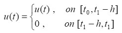

see Sebakhy and Bayoumi (1973). It is null controllable with constraints at t= t₁, if for any initial state {χ₀, χ_to, u_to} on [t_o - h, t₀] , there exists an admissible control u (t) ε U , defined on [t_o - h, t₀] such that the response χ (t) of system (3) satisfies χ (t) = 0 , using the control effort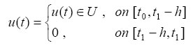

Definition 4 - The domain D of null controllability of system (3) is the set of all initial points χ₀ε Εⁿ for which the solution χ (t) of system (3) with χ (t₀) = χ₀ satisfies χ (t₁) = 0 ε Eⁿ at some t₁ using u ε U

Definition 5 - An operator T : X → Y, where X and Y are linear spaces, is said to be closed if for any sequence u_nε D(T) such that u_n→ u and Tu_n→ v, u belongs to D(T) and Tu= v .

The variation of parameter of system (3) for t>t_o + h imply the existence of a unique absolutely continuous solution χ(t) of system (3), with initial complete state z(t₀) of the form

where X(t,s) satisfies the equation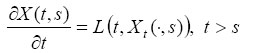

almost everywhere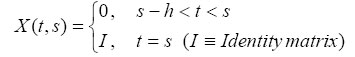

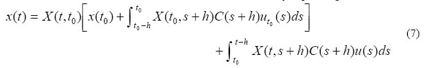
X (t, s) is called the fundamental matrix solution of the system

χ(t) = L(t, χ_t) (6)

We now obtain a more convenient form of the solution (3) by expressing (5) as

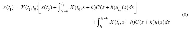
The solution χ(t) of system (3) at t = t₁ (Klamka, 1980) becomes

We now define the n x n controllability matrix of system (3), given by

Where T denotes transpose

Definition 6 - The reachable set of system (3) at time t₁ using L₂ controls is the subset of Eⁿ given by

and the constraint reachable set of system (3) is given by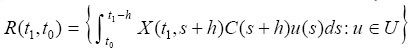

The constraint reachable set with unspecified end time is given by

Definition 7 - System (3) is said to be proper in Eⁿ 0n [t₀, t₁] if

C^t[X(t₁, s + h) C (s + h)] = 0

almost everywhere t ε [t₀, t₁], c ε En implies c = 0. If system (3) is proper on [t_o, t_o, + δ] for each δ. 0, we say system (3) is proper at time t₀. If system (3) is proper on each interval [t₀, t₁], t₁> t₀> 0, we say the system is proper in Eⁿ

NULL CONTROLLABILITY WITH CONSTRAINED CONTROLS

Lemma 1 - The following are equivalent

(i) W(t₀, t₁) is non singular for each t

(ii) System (3) is proper in Eⁿ for each interval [t₀, t₁]

(iii) System (3) is relatively controllable on each interval [t₀, t₁]

Proof - W(t₀, t₁) is non singular implies W(t₀, t₁) is positive definite, that is

C^t[X(t₁, s + h)C(s+h)]= 0

almost everywhere on [t₀, t₁] implies c = 0 . Therefore, (i) implies (ii).

To prove the equivalence of (ii) and (iii) let c ε Eⁿ, and assume that

C^t[X(t₁, s + h)C(s+h)]= 0

almost everywhere tε[t₀, t₁] for each t₁, then

for u ε L₂. It follows from this that c is orthogononal to the set P(t₁, t₀) . We assume that system (3) is relatively controllable, then P(t₁, t₀) = Eⁿ, so that c = 0 , meaning that (iii) implies (ii). Conversely, assume that system (3) is not controllable, so that , for t₁> t₀. Then, there exists , c ε Eⁿ, such that c^tP(t₁, t₀) = 0 .

It follows that for all admissible control u ε L₂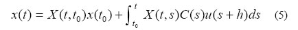

To show that (i) implies (ii)

We define the operator K :L₂ ([t₀, t₁], Eⁿ) → Eⁿ by

If we assume that W(t₀, t₁) is singular. Then the symmetric operator KKT =W(t₀, t₁) is positive definite. But this holds, if and only if rank W(t₀, t₁) = n.

Theorem 1 - System (3) is proper on [t₀, t₁] if and only if 0 εint R(t₁, t₀).

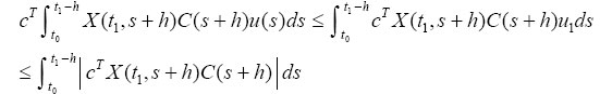
Proof - If R(t₁, t₀) is a closed and convex subset of Eⁿ (Klamka, 1976), then a point y₁ on the boundary of R(t₁, t₀) implies that, there is a support plane of R(t₁, t₀) through y₁, that is ct (y - y₁)≤ 0 for each y ε R(t₁, t₀) where is an outward normal to . If u₁ is the control corresponding to y₁, we have

for each u ε U . Since U is a unit sphere, this last inequality holds for each u ε U , if and only if

and u₁ (t) = sgn c^T (X (t₁, s + h) C(c+h)) as y₁ is on the boundary. Since we always have 0 ε R(t₁, t₀) . If ₀ were not in the interior of R(t₁, t₀) then 0 is on the boundary, hence, from the foregoing, this implies so that

c^T (X (t₁, s + h) C(c+h)) almost everywhere t ε [t₀, t₁] . This by our definition implies that the system is not proper since . This completes the proof.

Theorem 2 - System (3) is relatively controllable if and only if 0 ε int R(t₁, t₀) for each t₁ > t₀

Proof - By lemma 1, system (3) is relatively controllable on [t₁, t₀], t₁ > t₀ if and only if, it is proper on [t₀, t₁] . Therefore, by theorem 1, system (3) is relatively controllable if and only if 0 ε int R(t₁, t₀).

Theorem 3 - If system (3) is relatively controllable on [t₀, t₁] for each t₁ > t₀, then the domain null controllability of system (3) contains zero in its interior

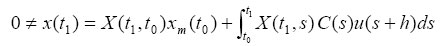
Proof - Assume that system (3) is relatively controllable on [t₀, t₁] , t₁ > t₀ then by theorem 2, 0 ε int R(t₁, t₀), for each t₁ > t₀. Since x = 0 is a solution of system (3) with u =0 , we have 0 ε D. Hence, If , then there exists a sequence such that x_m→ as m→ ∞ and no x_m is in D, that is xm ≠ 0 . From (5), we have

for any t₁ > t₀ and any u ε U. Hence, for u= 0 , ,

is not in R (t₀, t₁) for any t₁ > t₀. Therefore the sequence is such that , but z_m→ as m→ ∞. Therefore, a contradiction. Hence, 0 ε int D.

Theorem 4 - Assumes

(i) System (3) is relatively controllable on [t₀, t₁] for each t₁ > t₀

(ii) The zero solution of system (6) is uniformly asymptotically stable, so that the solution of (6) satisfies are constants. Then system (3) is null controllable with constraints.

Proof - By (i) and theorem 3, the domain D of null controllability of system (3) contains zero in its interior. Therefore there exists a ball B₁ such that . By (ii), every solution of system (3) (with u = 0 ) satisfies x(t) →0 as t → ∞ . Hence at some t₁< ∞ (with u = 0 ) , for t₁ > t₀. Therefore, using t₁ and x₁ = x(t₁) and _t1 at u = o as initial data there exists a u ε U and some t₂ > t₁ such that the solution x(t) of system (3) satisfies x(t₂). Thus proving the theorem.

Lemma 2

System (3) is relatively controllable on [t₀, t₁] if and only if rank W(t₀, t₁)= n .

The proof is quite standard and simple, for similar proof see Klamka (1976 ).

Theorem 5 - System (3) is null controllable with constraints if

(i) Rank W(t₀, t₁)= n , for t₁ > t₀

(ii) The zero solution of (6) is uniformly asymptotically stable

Proof - Immediately from theorem 4 and lemma 1

Theorem 6 - The system (6) is null controllable with constraints if

(i) Rank W(t₀, t₁)= n , for t₁ > t₀,

(ii) If all the characteristics roots have negative real part

Proof : Immediately.

Conclusion: In this paper we have developed and proved sufficient conditions for the controllability and null controllability of liner systems with delay in the state and control. That is, if the uncontrolled system is asymptotically stable and the controlled system is relatively controllable then, the system is null controllable with constraints.