|
| About Bioline | All Journals | Testimonials | Membership | News |
|
||||||
|
||||||
Journal of Applied Sciences & Environmental Management, Vol. 9, No. 3, 2005, pp. 71-76 Euclidean Null Controllability of Nonlinear Infinite Delay Systems with Time Varying Multiple Delays in Control and Implicit Derivative *1JACKREECE, P C; 2DAVIES, IYAI 1Department of Mathematic, Rivers State
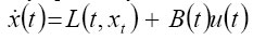
College of Education, Port Harcourt. E-mail; preboj@yahoo.com. Code Number: ja05061 ABSTRACT: Sufficient conditions for the Euclidean null controllability of non-linear delay systems with time varying multiple delays in the control and implicit derivative are derived. If the uncontrolled system is uniformly asymptotically stable and if the control system is controllable, then the non-linear infinite delay system is Euclidean null controllable. @JASEM The control processes for many dynamic systems are often severely limited, for example, there may be delays in the control actuators. Models of systems with delays in the control occur in population studies. Most specifically models of systems with distributed delays in the control occur in the study of agricultural economics and population dynamics, Arstein (1982), Arstein and Tadmor (1982). In most biological populations the accumulation of metabolic products may inconvenience a population and this result in the fall of birth rate and increase in death rate. If it is assumed that total toxic action in the birth and death rates is expressed by an integral term in the logistic equation then an appropriate model is the integro-differential equation with infinite delays. Several authors have studied these systems and established sufficient conditions for the controllability and null controllability of these systems, Chukwu (1992), Gopalsany (1992). Chukwu (1980) showed that if the linear delay system
is uniformly asymptotically stable and is proper, then
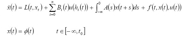
is Euclidean null controllable, provided f satisfies certain growth and continuity condition. Sinha (1985) studied the non-linear infinite delay system
and showed that (1) is Euclidean null controllable if the linear base system
is proper and the free system
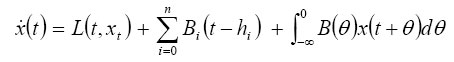
is uniformly asymptotically stable, provided that f satisfies some growth conditions. Balachandran and Dauer (1996) studied the null controllability of the non-linear system
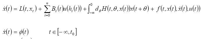
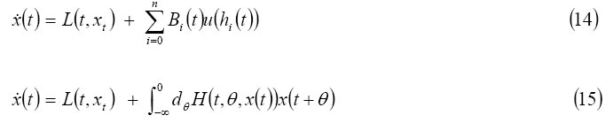
Hale (1974) provided sufficient conditions for the stability of systems of the form The aim of this paper is to study the null controllability of systems of the form
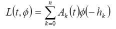
whereL(t, Ø) is continuous in t, linear in Ø, and is given by
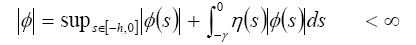
BASIC ASSUMPTIONS AND PRELIMINARIES. Let Enbe an n-dimensional linear space with norm |.| . In equation (6) Ai is a continuous n x n matrix function for 0 ≤ hi ≤ h and H (t, θ. x(t)) is n x n matrix valued function which is measurable in (t, θ. x(t)) , and H (t, θ. x(t)) is of bounded variation in ( θ, x(t)) in ( - ∞, ∞) The matrix function Bi(t) i = 2, 1, 2, ........n are n x p , continuous in t and h + t0 - mini hi(to) where h1 (t)are defined below. Here x ε En and u ε Ep. Let 0 ≤ h ≤ y be given real numbers (y may be + ∞). The function η : [- y, 0] → (0, ∞)is lebesque integrable on [- y, 0], positive and non-decreasing. Let B([- y, 0] En) be the Banach space of functions which are continuous. Let B([- y, 0] En be the Banach space of functions which are continuous and bounded on [-y , 0] such that
for
any t ε R and
any function
Assume that the function hi[t0, t1] → R i = 0, 1, 2, .........n are twice continuously differentiable and strictly increasing in [t0, t1], further
Let us introduce as in Kantorovich (1992) the following time lead function r1 with such
that hi(t)=tand for t=t1 the function hi(t) satisfies the inequalities
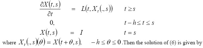
Let the fundamental matrix X satisfy the equation
with
initial state
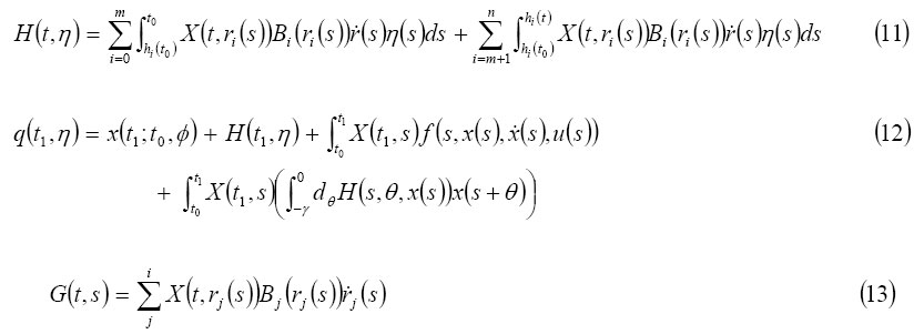
For brevity introduce the following notations
Consider the homogeneous systems
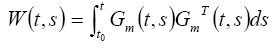
The controllability matrix of system (14) at time t is given by
where T denotes matrix transpose. Chukwu (1992), established null controllability of systems of the form (14) DEFINITION: The system (6) is said t o be null controllable if for each Ø ε B([- y, 0], En) there is a t1≥ t0, u ε L2 ([t0, t1])u is a compact convex subset of Ep such that the solution x(t; t0, Ø , u) of (6) satisfies xto(t; t0, Ø , u)= θ and x(t; t0, Ø , u)= 0 MAIN RESULT THEOREM: Suppose that the constraint set u is an arbitrary compact subset of Ep and that i.
Assume that system (15) is
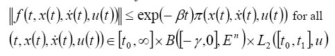
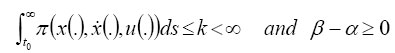
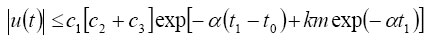
uniformly asymptotically stable, so that the solution ii. The linear control system (14) is controllable iii. The continuous function f satisfies
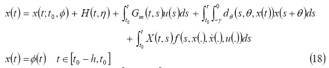
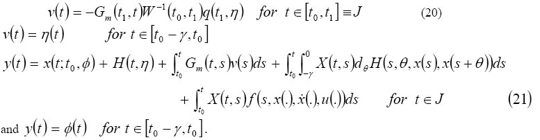
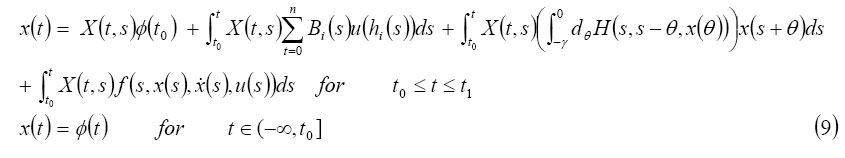
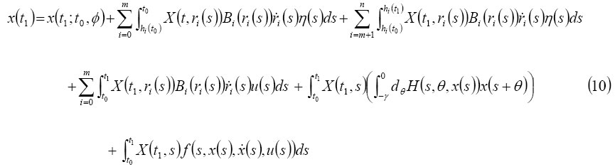
Where then (6) is Euclidean null controllable. Proof: Since (15) is controllable, hence it is proper in En exists for each w-1(t0, t1) . Suppose the pair of functions x, u form a solution pair to the following equations for
some suitable chosen
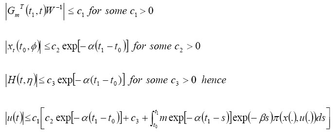
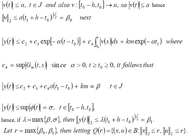
then u is square integrable on [t0 - h, t0] and x is a solution of (6) corresponding to the control u with initial state Y(to) = x(to; Ø , η) = 0. Now it is shown that u : [(t0, t1) ] → u is a compact constraint subset of En that is |u| ≤ a for some constant a > 0 Since (15) is uniformly asymptotically stable and Bi are continuous in t, it follows that and therefore since β - α ≥ 0 and s ≥ to ≥ 0. From (18) t1 can
be chosen so large that
It
remains to prove the existence of a solution pair of the integral equation (16)
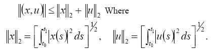
and (17). Let B be the Banach space of all functions Define the operation T : B → by T(x, u) = (y, v) where Because of the various assumptions on our system and the estimate from (17) to (19) it is clear that It follows that T : Q(r → Q(r)) since Q(r) is closed, bounded and convex, by Rieze’s theorem (Kantorovich and akilov, 1992) it is relatively compact under T. The Schauders theorem implies that T has a fixed point (x, u) ε Q(r), this fixed point (x, u) of T is a solution pair of the set of integral equations (20) and (21). Hence the system (6) is Euclidean null controllable. REFERENCE
Copyright 2005 - Journal of Applied Sciences & Environmental Management |
| |||||||||


 (4)
(4) (5)
(5) (6)
(6) (7)
(7)
 (8)
(8)
 (16)
(16)