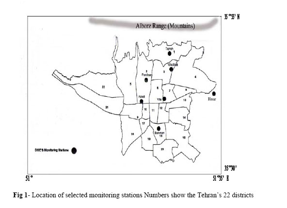
Journal of Applied Sciences & Environmental Management, Vol. 10, No. 2, 2005, pp. 75-82 

Study on the Status of SO₂ in the Tehran- Iran

^1*ELHAM, ASRARI; ²GHOLE, V S; ³SEN, P N

¹Departmentof Environment- Tehran, Iran
²Departmentof chemistry, University of Pune, India
³Departmentof Atmosphericand Space Science, Universityof Pune, India E-mail:elasrari @yahoo.com

Code Number: ja06028

ABSTRACT

An air quality analysis for Tehran, the capital city of Iran, is conducted for SO₂, with the measurements taken from 1995 to 2002. Measurements were taken from the seven main monitoring stations in different locations of the city. These stations are controlled by Department of Environment of Iran. As a first step; annual, seasonal and diurnal variations were studied. The yearly variation does not show any specific trend initially but in the recent years it seems there is a little upward trend. The pick of concentration of SO₂ can be seen during 6-12 hour and during the winter season especially in January. The main purpose of this study is to see the effect of the meteorological parameters on the concentration of pollutant. For this purpose, the wind velocity, relative humidity, temperature, dew point, wind direction and rainfall are considered as independent variables. The relation between concentration of pollutant and meteorological parameters can be expressed by one linear regression equation. It is obvious from the equation that the wind speed, daily temperature and humidity have reverse effect on the concentration of SO₂. To plan and execute air pollution control programs, one must predict the ambient air concentrations that will result from any planned set of emissions. For this purpose, a two-dimensional atmospheric diffusion model for ambient air concentration of SO₂ was considered. Geostrophic winds, surface roughness, mixing height of the atmosphere, emission rate of the pollutant sources and background pollutant concentration have been taken as the input parameters. The airspace over the city to the mixing height was divided into multiple cells. Conservation of mass equations for each cell were solved for slightly stable and highly stable atmospheric conditions of city. The results of this equation were adjusted by the actual data (taken from monitoring stations). Then the modified dispersion equation for concentration of SO₂ in Tehran has been suggested. @JASEM

Air sustains life. But the air we breathe is not pure. It contains a lot of pollutants and most of these pollutants are toxic. SO₂ is the one of the five primary pollutants which together contributes more than 90% of global atmospheric pollution (Sharma 2001). The presence of pollutants in the atmosphere, causes a lot of problems, thus the study of pollutant’s behavior is necessary. Status of pollutants concentration and effect of meteorological and atmospheric parameters on it is the base of such studies as follows: Semi-statistical model has been studied for evaluating the NO_x concentration by considering source emissions and meteorological effects by Lin and Wu (1994). Street level of NO_x and SPM in Hong Kong has been investigated by Lam et al (1997). The progressive decrease of air pollution from west to east in Kolkata has been shown by Mandal (2000). Statistical modeling of ambient air pollutants in Delhi has been used studied by Chelani, et al (2001). Also for predicting co, Sabah A. et al in 2003 used a statistical model. Influence of meteorological factors on air pollution was researched by Gupta et al (2004). Atmospheric diffusion models are being widely used to study the complicated relationships between air quality and emission sources conditions. In general, these models are based on the equation governing the pollutant concentration consistent with the physical principle of mass conservation. McRae and Seinfeld (1983) developed mathematical model for urban air pollution. Nokes et al (1984) developed a model to study turbulent dispersion of steady two dimensional horizontal sources. Piedelievre et al (1990) studied an eulerian model of atmospheric dispersion. A Two-dimensional Lagrangian dispersion model was improved for daytime conditions by Rotach et al (1996). Berkowicz et al (1996) used measurements of air pollution in streets for evaluation of urban air quality, meteorological analysis and model calculations. A research project for observation and modeling of urban air pollution in UK west midlands was done by Harrison et al (2000). Hanna et al (2003) studied urban dispersion model evaluated with Salt Lake City and Los- Angeles tracer data.  The research area, Tehran is the capital of Iran which is located between 35° 35' N and 35º 50' N latitudes 51° 05' E to 51º 35' E Longitudes and the elevation is 1280 m above the mean sea level. Area of Tehran is 730 km². It has moderate climate and residential population in 2001 was7195093. The biggest environmental problem which Iran currently faces is air pollution, especially in the capital city of Tehran. About 1.5 million tons of pollutants are produced in Tehran annually. Most of the cars are over 20 years old, with poor fuel efficiency and lacking catalytic converters and the ability to use lead-free gasoline Leaky engines. Vehicles spewing black smoke are a familiar sight contributing to the city's hazardous air pollution, as well as its infamous traffic snarls. Tehran's air pollution is made even worse by the city's geographic position. The city is hemmed in by the Alborz Mountains to the north, causing the increasing volume of pollutants to become trapped, hovering over Tehran when the wind is not strong enough to blow the pollutants away.

Tehran's high altitude, ranging between 1006 and 1524m, also makes fuel combustion inefficient, adding to the pollution problem.  Finally, the city's "lungs" (i.e., its orchards, especially in northern Tehran) have largely been destroyed over the past 10-20 years by rampant development pressures.  The combination of these natural and man-made factors have made Tehran as one of the most polluted cities in the world, ranking with Mexico City, Beijing, Cairo, Sao Paulo, Shanghai, Jakarta, and Bangkok.  Hence a need was felt to carry out an ambient air quality monitoring in Tehran and also the analysis of ambient trends can indicate the adequacies or deficiencies in emission inventories and emission reduction estimate.

Materials and Methods  

Seven different sampling stations Azadi, Tajrish, Gholhak, Bahman, Hesar, Vila and Pardisan were selected from different parts of the city (fig 1).

The sampling has been done every 30 minutes every day for each pollutant by monitoring stations. The instruments that use in these stations are Horiba .The first monitoring station was established in 1995.This instrument (Horiba) can be used for a wide variety of analyses and tests for continuously monitoring some of pollutant concentrations in ambient air. The instrument can simultaneously measure concentrations of those pollutants (SO₂, NO₂, dust, CO, O₃, NO, NO_X etc). The instrument may be calibrated automatically or manually. Among measured data SO₂ was chosen for the seven stations. Then the averages were calculated for every six hours, each month and each year for every station to understand the status of concentration of SO₂ from past to the present. At last the average of data has been used for the analysis. The next step was to find the correlation of the concentration of SO₂ and metrological parameters. Software of SPSS has been used for this purpose and thelinear regression equationshows that the concentration of SO₂ with the meteorological parameters and also gives an idea about the levels of this relation. Finally the basic equation of conservation for SO₂ concentration in the presence of turbulent diffusion has been used for suggesting dispersion model by using the K- theory approach.  The basic equation (1) is:

C = the mean pollutant concentration in the air at any location(x, y, z) at time t; u, v, w = the x, y and zcomponents of the mean wind velocity respectively; K_x, K_y and K_z = The eddy diffusivity coefficients in x, y and z directions respectively; u, v and w = the components of the mean wind velocity; K_x, K_y and K_z = the eddy diffusivity coefficients in x, y and z directions;  S= source term;  R= removal term

We assume that the urban area is a single source of air pollution, the pollutant are chemically inert, the pollutant does not have any of the removal mechanisms such as dry deposition, gravitational setting etc, the total emission in an urban area is treated as uniformly distributed, SO₂ is confined below the mixing height, horizontal advection is greater than horizontal diffusion for not too small values of wind velocity, the concentration of SO₂ does not vary in crosswind direction (No y- dependence) ,vertical diffusion is greater than vertical advection since the vertical advection is usually negligible compared to diffusion owing to the small vertical component of the wind velocity and neglecting time dependency ,the equation (1) reduces to:

With these boundary conditions                       

u = u (z) is the mean wind speed in the x direction

C = C(x, z) is the ambient concentration of the pollutant

K _z = k _z (z) is the turbulent eddy diffusivity

Q=Q(x) is the emission rate of the pollutant 

B= B (z) is the background concentration of the pollutant

z _mix= the mixing height

L = Desired distance

l = Source extension. 

A numerical method of solving equation (2) is as follows:

The space over the city divided to boxes then for each box the conservation of mass was used. For example the mass of pollutant came into the first box is u₁Δz B₁ (Δx, Δz and 1 unit are wide, high and deep of each box respectively) and the mass advected out of the first box is u₁Δz C₁. The mass flux per unit area added to the first box is Q Δx. The mass diffusion out of the first box is k_z1 Δx (C₁-C₂)/ Δz. For all of the boxes the mass equations can be written. Then all the equations can be rewritten in the matrix notation as:   [A _ij] [C_j ] = [D_i]

The A   matrix consists of terms due to the advective and diffusive fluxes into and out of the boxes. The D matrix consists of the known mass flux into the boxes. The concentration of pollutant, C, is found by solving the matrix. Conservation of the concentrations in the horizontal row of boxes is referred to as the ground level ambient air concentration (μgm^-³).This calculation has been done for January, April, July and October.  For solving equation (2), we should know realistic form of the wind and eddy diffusivity which are functions of vertical distance.

In this case by considering the atmospheric condition for the Tehran city(JICA1997), slightly stable and highly stable conditions as a critical status of the atmosphere in the city have been chosen. For solving equation (2), eddy diffusivity and wind velocity profile should be obtained. The atmospheric stability in the boundary layer is generally characterized by the parameter L (Monin and Obukhov, 1954), which has the unit of length and is given by (eq3):

 u _* =  The friction velocity;  H = the net heat flux; ρ =   The ambient air density;  c_p =   specific heat at constant pressure; T =   the temperature;  k =   Von Karman constant (=0.4)

 g = the gravitational acceleration.

The friction velocity is defined in terms of geostrophic drag coefficient (C_g) and geostrophic wind (u _g) as (eq4):                 

u _* = C _{g *}u _g        (4)

C_g is a function of the surface Rossby number (R₀= u _* /f z₀) and f is the Coriolis parameter of the earth and z₀ is the surface roughness. Lettau (1959) suggested the following expression for C_g for a neutral atmosphere (eq5):         

C_g = 0.16/ [log (R₀) - 1.8]     (5)

For the purpose of this model, the following scheme is used:

Unstable flow:                   c_g = 1.2Cg (neutral)

  Slightly stable flow:          c_g = 0.8 Cg (neutral)

    Highly Stable flow:            c_g = 0.6 Cg (neutral))

For the computation of the eddy diffusivity the following relationships are used for the eddy viscosity in the planetary boundary layer above the surface layer (Ragland 1973):

For neutral stability with z> k u_*/f                                 K_M = k² u_*²/f

For stable flow with z> 6L                                K_M= 6k u_*L / (1+α)

For unstable flow with z>k u_*/f                         K_M=k u_* (1- 15k u_*/f L) ^{– 0.25}

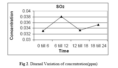
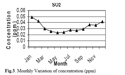
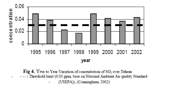
Because both the mass and momentum are transported by the turbulent eddies, it is physically reasonable that the ratio k _z / k _M remains constant and is equal to unity, at least in the surface layer and also  = 5.2, as shown by Webb (1970). Within the surface layer of the atmosphere, the wind speed has been determined by Ragland (1973)(eq 7):  

u= (u _g –u _{s L}) (z – z _{s L} / z _m – z _SL) ^p + u _{s L}                           (7)

u _g    =   geostrophic wind

u_sl   =   wind at z _SL

Z _{s L} =   the top the surface layer

Z _m    =   the mixing height, Z _m= 2300u_*^1.5

P      =   an exponent which depends upon the atmospheric stability

Value of the exponent (p) has been obtained from urban wind profiles, as suggested by Jones et al (1971).

      p= 0.2 for unstable and neutral condition

      p = 0.35 for slightly stable flow

      p= 0.5 for highly stable flow

For surface roughness, Z₀ is estimated 220 cm as average of city land use according to EPA report (1995). The source strength was calculated for SO₂ according to fuel consumption. And for realizing the effect on geostrophic wind on concentration pollutant the different u_g has been used.

The concentration of SO₂ is achieved from this equation. This amount is compared to the observed data from monitoring station. Although the data were not exactly same but the trend of variation was similar. Adding one constant to equation (2) one more equation is obtained for the predication of concentration of SO₂ with at least error (the equation can be seen in results).

Results and Discussion

In figures 2, 3 and 4, the diurnal, monthly and year to year variation of concentration of SO₂have been presented. The concentration of SO₂ is the highest during the period 6 to 12 hours (fig 2). A thermal power plant based on oil and coal contributes more than 60% of all sulfur oxides and 25-30% nitrogen oxides. In the morning their activity increase then the level of concentration of SO2 shows more amount than night. Figure 3 shows that monthly concentration of SO₂ is high during the winter months (January and February).The yearly concentration level of So₂ is showing up and down trend during the period of study and actually it is obvious that the amount is more than the tolerable limits. In winter inversion is observed in the city many times and it causes the concentration of pollutant to increase in the city. As can be seen in the figure 1, the north part of the city is Alborz rang and the effect of this can be seen when the average of concentration of pollutant among the monitoring data compare. Two monitoring stations, Tajrish and Golhak are located in north part of the city and the more amount of concentration of pollutant can be observed in these sites. After that, Azadi monitoring station (in the west of city) shows the more amount of pollution. The most concentration of pollutant can be observed in north, west, middle, southern and east of the city respectively.

At the next step linear regression equation involving one or more independent variables that gives best fit for the concentration of dependent variables has been found out.   Table 1 shows the relationships between SO₂ and metrological parameters. In table 2, the coefficient of pollutant model and regression line is presented. The linear model equation is as follows:

SO₂= (-0.002) Daily temperature + (-0.002) mean FF + (-0.0045) Humidity + 0.108

Prediction Intervals is between 0 to 0.1 ppm

Mean FF = Wind speed (ms^-1)

Among the meteorological parameters, daily temperature, wind speed and humidity have more effect on concentration of SO₂.The linear regression equation works well when the concentration of   SO₂ is between 0 to 0.1 ppm. These parameters have reverse effect on concentration of SO₂. It means the concentration of SO₂ increases by decreasing the wind speed, daily temperature and humidity. The concentration of SO₂ increases in January and

decreases in the July, the most effective meteorological parameter on concentration of SO₂ is daily temperature then during cold month (January) the concentration increases and in hot month (July) decreases. 

Mean FF = wind speed; Max DD = wind direction;  Daily tem = Daily temperature

Table 2 Value of Liner model coefficients for SO₂

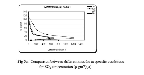
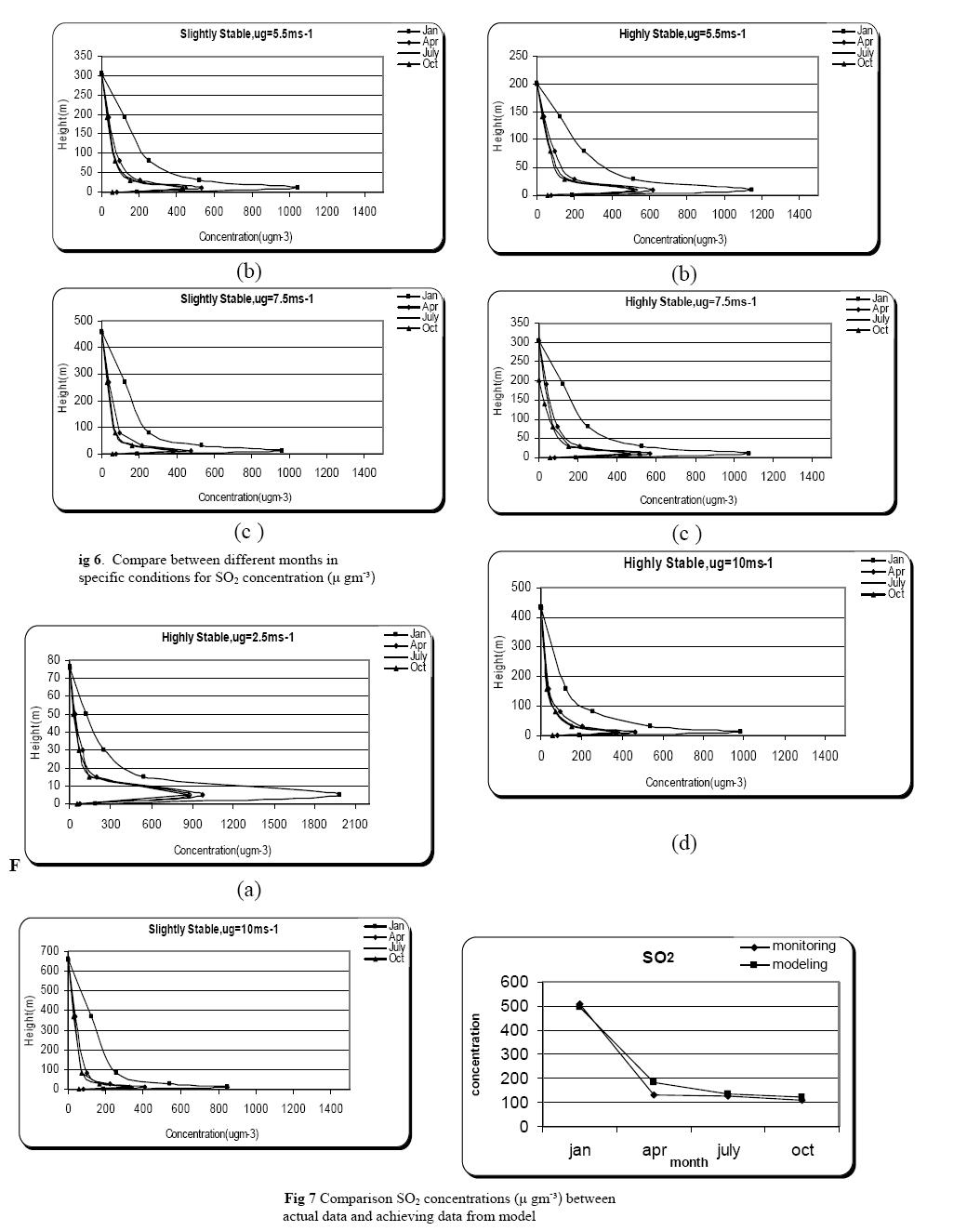
It can be seen also from figures 2, 5 and 6 that during January (the coldest month in the city) concentration of pollutant shows the highest amount.  At last the atmospheric dispersion model discussed previously now will be applied to real conditions and the result is this equation:

The model permits the estimation of concentration distribution for more realistic meteorological conditions. In the figures 5 and 6 comparison between difference of concentration of SO₂ and height in different seasons are shown.  figures 5 and 6 show that when geostrophic wind increases, the concentrations of pollutant decrease. In highly stable condition the pollutant concentration is more than that in slightly stable. In every type of atmospheric condition by increasing geostrophic wind, the height over the city that has the more pollutant concentration has been decreased but the extension of this amount increased.

When geostrophic wind increases, the height to which, the pollutants can penetratedecreases.Also the pollutant concentration increases as the distance within the source increases and decreases rapidly beyond the source. The comparison between actual data and modeling data can be seen in the figure 7. This model can be used to find the trend of changing SO₂ concentration and prediction.  Urban air pollution modeling is a complex forecasting problem and one or two assumptions are not sufficient to cope with it. If dispersion model has to play a useful role in urban planning or in devising pollution control strategies, it is necessary that reliable models of atmospheric dispersion is available .This developed dispersion model can be used for Tehran city. The advantage of this model is simple application because it doesn’t contain of complex equation. It can be used easily to predict and control the status of SO₂ in the city.By considering this model, the concentration of pollutants can be studied with present and absence of source; like urban centers and outskirts. Tehran’s future begins today and tomorrow will be too late then some suggestions like banning of old technology of vehicles and industries, increasing public transfer facility, extending network of the metro in the city, encouraging the industries to obey the standards of air quality, controlling traffic, controlling automobile factory for upgrading technology and using up-to-date standard to design engine and more for conserving the environment of the studied area against the air pollution can be adopted by the local government for enforcing the existing laws for environmental conservations.

References