 |
| About Bioline | All Journals | Testimonials | Membership | News |
|
||||||
|
||||||
Iranian Journal of Environmental Health, Science and Engineering, Vol. 8, No. 2, 2011, pp. 139-152 Simulation Of Temperature Changes In Iran Under The Atmosphere Carbon Dioxide Duplication Condition *Gh. R. Roshan, F. Khoshakh lagh, Gh. Azizi, H. Mohammadi 1Faculty of Geography, Department of Physical Geography, University of Tehran
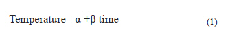
Received 12 April 2010; revised 23 October 2010; accepted 18 December 2010 Code Number: se11017 ABSTRACT The present research intends to show the effect of global warming on the trend and patterns of temperature in Iran. The study has been divided into two primary parts, the first of which is an analysis of the country's temperature trend using the following data measures: the minimum, maximum, and mean seasonal night temperature (the minimum temperature) components, the day temperature (the maximum temperature) component and the mean daily temperature component. This data is specific to the time frame 1951 to 2005 and it was obtained from 92 synoptic and climatology stations around the country. The second part of this research involved simulating and forecasting the effects of global warming on temperature values under conditions in which greenhouse gases have increased. For analyzing these simulations and forecasts the MAGICC SCENGEN model was used and different climate change scenarios were taken into consideration. The results are quite interesting. In the analysis of the country’s current temperature trend and in the forecasting’s, specifically related to time, a significant temperature increase was observed during the summer months. Also, with regard to altitudinal levels, it was evident that stations at higher altitudes show a more significant increase in daily and mean daily temperatures. Taking into account the output mean of the different climate change scenarios, the temperature simulations show a 4.41° C increase in Iran’s mean temperature by 2100. Most of these temperature increases would occur in the southern and eastern parts of Bushehr, certain coastal regions of the Persian Gulf, eastern and western parts of Fars, Kohgilooye, Boyerahmad, southern parts of Yazd, as well as southern and southeastern parts of Esfahan. Key words: Simulation; Global warming; MAGICC SCENGEN; Carbon dioxide; Iran INTRODUCTION The development of urbanism and the expansion of cities, coupled with the rapid increase in population and intensification of industrial activities, has led to irregular patterns of consumption of fossil fuels. The consequent of this has been a massive output of pollutant by-products that firstly threaten city inhabitants with respiratory and intensified cardiovascular diseases, and secondly would act as an aggravating element in climatic fluctuations and environmental effects (George, 2007; Chappelka, 2007; Shakoor et al., 2008, Roshan et al., 2009; Makhelouf, 2009). Climate change and global warming has become a primary concern of scholars in the natural sciences, particularly climatologists and the environmentalists. This is understandable since these processors are sure to have an impact, of varying degree, on environmental and human activities and certain phenomena (Paoletti et al., 2007; Bytnerowicz et al., 2007; Roshan et al., 2009). In the past decades, political and scientific societies have conceded that human activities ‘might’ induce climate change. Today, scholars believe that the human role in the excitation of the greenhouse effect is undeniable. This, however, is not to lay claim to the notion that the greenhouse effect is an incident restricted to the recent past years, but rather to suggest that the process has manifested itself more clearly as a result of the increase in greenhouse gases which can be attributed to the activities of the recent past years. The most significant of these greenhouse gases to be discharged into the atmosphere is CO2. Paleontological studies have shown that CO2 concentration existing in the earth’s atmosphere has fluctuated between 200 to 300 parts per million (ppm). During the past until 150,000 years ago, and again in the previous millennium the concentration of CO2 has been 280 ppm. Since 1990, CO2 levels began to dramatically increase in tandem with the start of the industrial revolution, the irregular consumption of fossil fuels, deforestation and the destruction of pasturages especially in rainy torrid zones. In 1990 the concentration of CO2 was 353.82 ppm, in 2000 this fig we reached 368 ppm. These increases in CO2 levels coincided with increases in global temperatures (IPCC, 2001). The International Panel of Climate Change (IPCC) has offered different scenarios in forecasting outcomes wherein there exists a sustained increase in greenhouse gas emissions. In this study it is assumed that CO2 concentrations would double by the end of the 21st century. In scenarios B, C, and D, proportionate to the control level of the greenhouse gases, the concentration of CO2 would be doubled accordingly in 2040, 2050, and by the end of the 21st century. The general circulation models and the quantitative weather forecast models originated from a similar source in the 1950's. The purpose of constructing these models is to simulate all three dimensional characteristics of climate. They are not only inclusive but also the most complete atmospheric models and therefore a reliable method for forecasting (Roshan et al., 2010). Among many phenomena that influence climate change, temperature functions as one of the most critical elements. It is a fundamental constituent of climate, and changes in temperature can dramatically alter the climate structure of a place. This in part explains why the study of temperature trends, specific to different time periods and local criteria, forms a major part of climatology literature. Studies have shown that during the last century there has been a marked increase in temperature in most parts of the world. Niedzwiedz et al. (1996) studied the day and night temperature trend in central and southeast Europe. Grieser and colleagues (2002) looked in to the temperature pattern of Europe over a period of one hundred years and found that the annual temperature cycle has been deferred in the west of Europe and has been held forward in the east of Europe. In the east of Europe, the annual fluctuation of temperature indicates a significant increase and in most of the regions the temperature has an increasing trend. Kaus and colleagues (1995) piloted temperature trend models for most northern countries- by studying the daily range and cloudiness peculiar in these countries and was than able to forecast the temperature of these regions . Koutyari and colleagues (1996) studied the temperature and precipitation trend in India. Yin (1999) studied the winter temperature disorders of the northern fields of China and explained its relation to the patterns of atmospheric currents outside the Torrid Zone. (Zhang et al., 2000) examined both temperature and precipitation trends in Canada over the 20th century. Salinger (1995) investigated the night and day temperature trends in the southwest region of the Pacific Ocean. Yue and colleagues (2003) studied the monthly, seasonal, and annual temperature trends of Japan over the past one hundred years. They found, using the Mann Kendall test that the annual temperature trend has increased from 0.51°C in 1900 to 2.77°C in 1996. Many academics researching and tracking the changes of certain constituents of climate, and in particular temperature, are reliant on Global Circulation Models (GCMs). Due to the curious effect global warming has on temperature scholars have tried to simulate and predict, for varied time periods, the degree of temperature change for different parts of the world (Gregory et al., 2000; Huybrechts et al., 2004; Lucio, 2004; Stössel et al., 2006; Goubanova, 2007; Krewitt et al., 2007; Laurent et al., 2007; Rowshan et al., 2007;Hertig et al ., 2008; Tolika et al., 2008; Haywood et al., 2009; Skeie et al., 2009; Chust et al., 2010). In Iran, research has been conducted on the changes in the temperature trend of different regions. Masoudin (2005) has studied Iran’s temperature trend for the past fifty years, and he has found that the night, daily, and 24-h temperature variables have respectively increased by 3°C, 1°C, and 2 °C in every one hundred years. These increases in the temperature trend have been most prominent in lowlands and in hot areas. Having studied the climate changes in the southern part of the Caspian Sea, Azizi and Rowshani (2008) came to the conclusion that at most of the stations, the minimum temperature had a positive trend, while the maximum temperature had a negative trend and thus the temperature fluctuation range had decreased. Mohammadi and Taghavi (2005) studied the precipitation and temperature limit indices in Tehran. In another study, Roshan and colleagues (2010) studied the horizontal expansion of Tehran and its effect on climate change. The results of their study suggested that there have been some changes and fluctuations in climate components particularly within the past decade. These changes have led to a more favorable and warmer climate condition in Tehran. In a study by Koochaki and colleagues (2003) the researchers explored Iran's climatic changes based on the duplication of carbon dioxide. In their study, they used the Geophysical Fluid Dynamics Laboratory (GFLD) model. The results indicated that when atmospheric carbon dioxide was doubled, the country's temperature increased. This increment was more evident in the northern and western parts of the country and also more prominent during spring and summer months. Salahi and colleagues (2007) used the General Circulation Model (GCM) to simulate the precipitation and temperature trend of Tabriz under conditions in which atmospheric CO2 had been doubled. Due to the importance of global climate change and its effect on temperature, this article intends to assess and track changes in Iran’s temperature trend over the past decades. Also, using the MAGICC SCENGEN model, it aims to simulate and forecast the country’s temperature under the conditions of global warming. MATERIALS AND METHODS This study includes two major and principal parts; the first part is related to analysis of the country's temperature trend by the use of the existing data. To evaluate Iran's temperature trend using the available data, the minimum, maximum, and mean seasonal night temperatures (the minimum temperature), day temperature (the maximum temperature), and the 24-hour temperature (the mean temperature) of 92 synoptic and climatological stations from Jan.1951 to Dec. 2005 have been used. For more precise and inclusive study of the entire country and in order to be able to use more stations, the minimum base statistics of 20 years has been selected. The trend tests are classified into two parametric and nonparametric groups. The presupposition of the parametric tests is that the data are random and outcomes of a normal distribution. Still, the presupposition of normality of the data does not exist in the nonparametric tests. Therefore, in case the normality of the data is not reliable, it is more confident to use nonparametric tests. Notwithstanding, some researchers have proved that the difference between the results of the two methods is not significant in regard to many of the climate components (Masoudian, 2005). Here, for the purpose of performing the temperature trend test, it was supposed that temperature is a linear function of time; therefore, the changes model would be as follows (Eq.1):
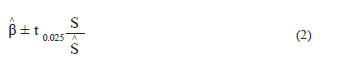
It is evident that a positive value of β indicates the temperature increase by time, and a negative value for β indicates the temperature decrease by time. If β=0 the presupposition is not proved. But since the value of β is definite, an estimation of β is obtained from the following equation with 95% of reliability (Masoudian, 2005):
If the upper and the lower limits of β, obtained by this method, are both positive, the presupposition of increasing trend of temperature is not rejected. If the upper and lower limits of β are both negative, the presupposition of decreasing trend of temperature is rejected. If one of the upper or the lower limits is positive and the other one is negative, the trend presupposition is not confirmed. This test is performed separately on the raining time series of each season of a year. The second part of the research included forecasting and simulating the global warming effect on values of temperature component in the future decades. This part of the research has been performed for the purpose of simulating and studying Iran temperature changes under the condition of increased greenhouse gases. The data related to temperature of Iran from 1961 to 1990 has been selected as the base data, and the temperature changes for the future decades have been studied according to different scenarios. For the purpose of forecasting and simulating temperature parameter changes as a result of greenhouse gases dispersion increase, the MAGICC SCENGEN compound model has been used in this research. Since the temperature parameter in the model applied in this study is defined till 1990, using the data of these parameters for the years after 1990 is restricted and impossible. Therefore, this base data has been considered for the years before 1990. In this research, four different scenarios (B1ASF, A1ASF, B1AIM, and A1MES) have been used based on which the temperature parameter changes have been assessed. The scenarios used in this research are the IPCC suggested scenarios. These scenarios in fact offer an image of the future. In other words, these scenarios help to assess the future progressions in a complex system which is unpredic table in nature. Each of the scenarios is explained separately hereunder: Scenarios of A1 family The hypotheses of these scenarios are mainly based on the followings:
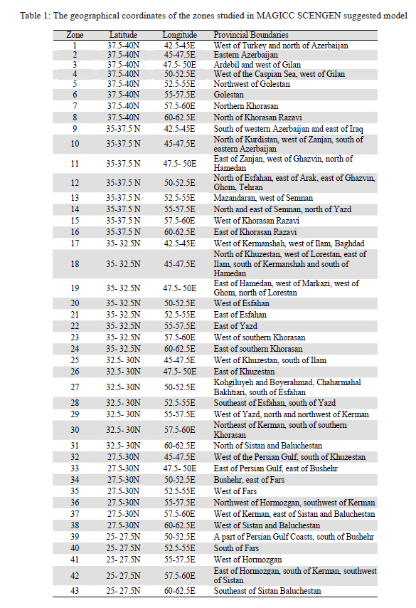
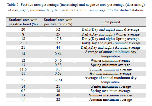
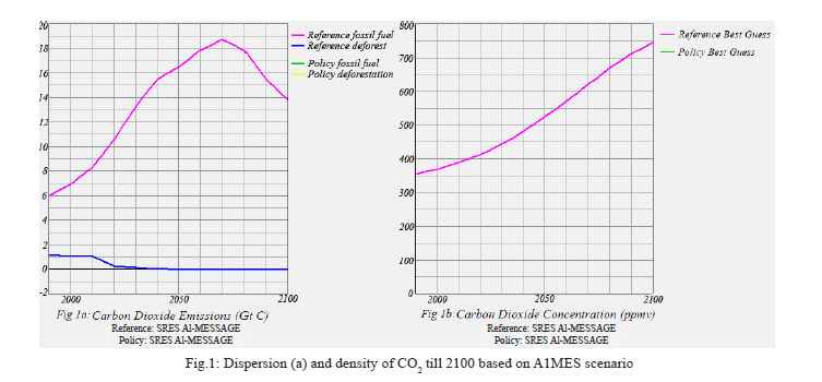
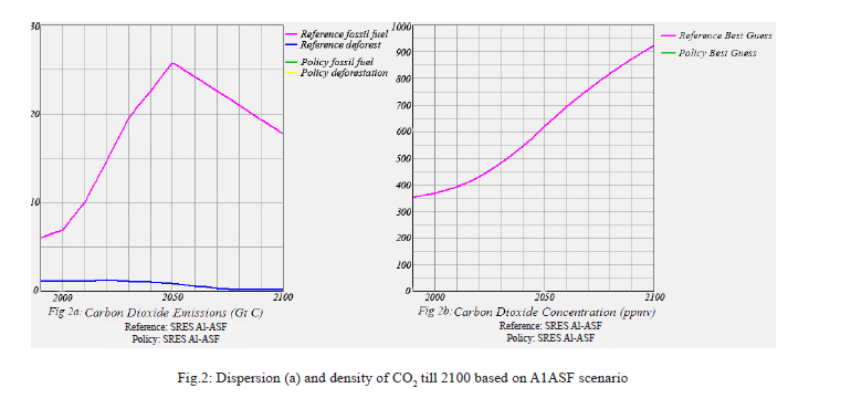
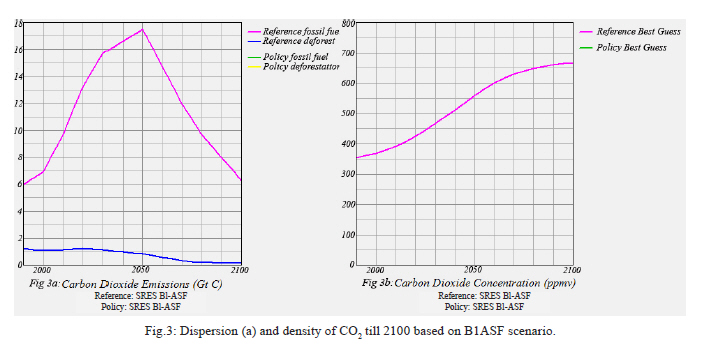
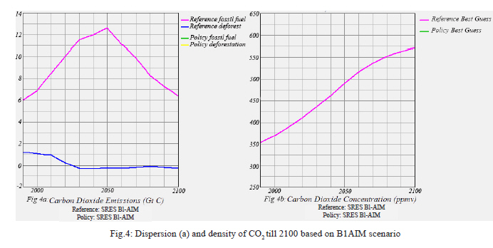
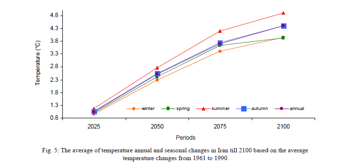
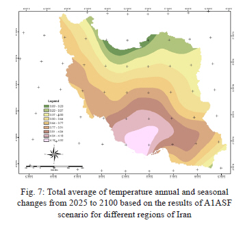
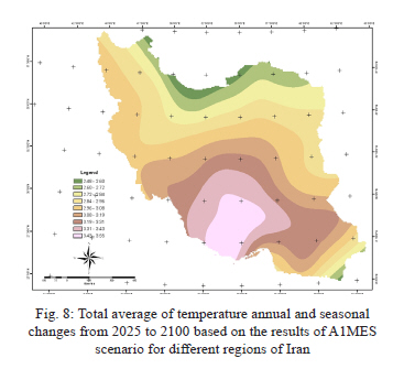
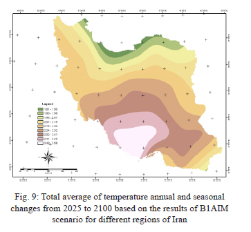
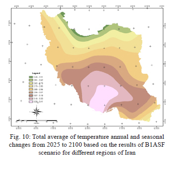
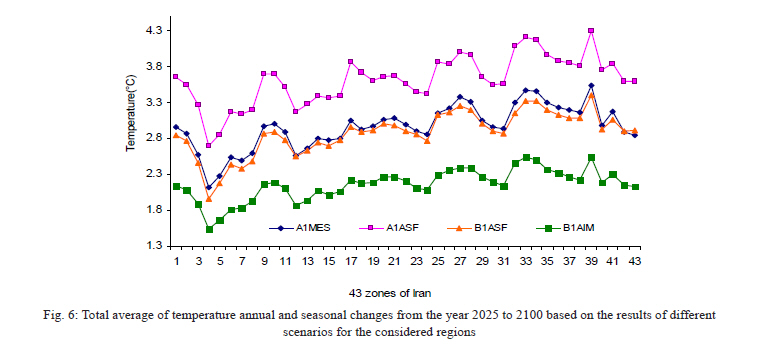
Scenarios of A1 family reflect the ambiguities in the field of energy resources development and technological changes in the changing world. Scenarios of B1 family The main element of this family is based upon the principal that the future will enjoy a great deal of social and environmental awareness aiming at stable development, and on this basis, it tries to forecast the future ambiguities. In better words, based on the scenarios of this group, the governments, the businessmen, the media and the people will pay more attention to environmental and social aspects of development (Moghbel, 2009). Structure of MAGICC SCENGEN Model MAGICC is a model for assessment of gas-induced climate changes and is comprised of a set of simple interrelated models. This model makes use of some parameters as input in the simulation process, the most important of which is climate sensitivity. The fact is that this model is used for the purpose of forecasting and simulating climate parameters with regard to these inputs for the future years and for different regions. In fact, MAGICC is not a GCM model but it uses the data of some climate models to simulate GCM models behavior for the considered region. In other words, this model is composed of a gas cycle as well as snow melting models which allows the user to determine the average global temperature changes and the datum level changes according to greenhouse gases dispersion (Wigley, 1996, 2000 and 2006). SCENGEN is a regional and global Scenario Generator. This model is not only a climatic model but a simple database including results of many GCMs as well as a set of global perceptional data and four sets of regional climate data. The fact is that SCENGEN is a simple software which allows the user to make use of the results of MAGICC model and the (GCMs). It also provides the ground for the user to recognize the consequences using different presuppositions in regard to climate system parameters. The scenarios of this model are in fact forecasted from dispersion of greenhouse gases in the future, using different hypotheses in relation to human activities, policies, and technology applications, etc. (Kont et al., 2003). By this method 20 GCM models can be used separately or in groups. In case of selecting several GCM models, the program averages them and produces a compound model of climate change (Moghbel, 2009). In the calculations performed for Iran, the average of the results of the two models (GFDLCM20, and GFDLCM21) was used. These models are two of the models of the geophysical flux dynamic laboratory of Princeton University. They are in possession of cloud schemas with interaction and shading variable over seasons. In another type of this model, known with R15 postfix, the atmospheric component has 9 levels in sigma coordinates and makes use of finite difference method on normal direction to solve equations. This version of the model is performed in a rhombic separation with 15 wavelengths in a complete orbit which is equal to 4.5x7.5 degree (length by width). The oceanic model has a 3.7x4.7 degree separation and 12 levels in normal direction. This model includes the sea ice dynamic model which gives additional freedom to the grading system. The deviation of the global mean temperature over the 1000-year simulation is very small (about -0.023 ° C in a century). Also this model has a discrimination power of 2.5 x 2.5 degrees. Regarding the fact that Iran is located in 25 to 40 degrees northern latitude and 44 to 63.5 degrees eastern longitude, and considering the mentioned discrimination power, Iran was divided into 43 geographical zones, and the temperature parameter changes have been simulated for each zone. It is also to be mentioned that the provinces located in the west and northwest part of the country are not included in the area with discrimination power of 2.5 degrees. Table 1 presents the 43 studied zones. The results of this model for temperature in 2025, 2050, 2075, and 2100 have been analyzed. RESULTS Study of the night temperature in different seasons in Iran indicates that summer, including 70% of the area of the stations, has the maximum number of stations with a significant increasing trend, while spring, autumn, and winter have the next ranks (Table 2). The results of Masoudian's study (2005) on Iran's temperature trend confirms the fact that in hot seasons a broader area experiences night temperature increase, while in springs, including 13% of the total area of the studied stations, the significance of temperature decrease in different stations is more evident so that the spring nights experience a higher decrease of temperature. After spring, this temperature fall is ranked consequently for winter, summer, and autumn. In studying the stations of the northern and the southern coasts of the country, the utmost significance trend of night temperature is observed in the southern coasts. In other words, increase of the southern coasts temperature is not due to increase of input radiation which determines the day temperature, but it is due to decrease of output radiation which determines the night temperature. Output radiation is influenced by the value of greenhouse gases in the atmosphere from among which water vapor has the most effect. Since the southern coasts have access to larger water resources located in lower latitudes receiving much input radiation leading to more evaporation and perspiration and increase of atmospheric humidity, a temperature increase follows this atmospheric humidity increase. On the other hand, in southern coasts which are under the effects of Azure High-Pressure influence in the major part of a year, especially in hot period, this factor leads to more humidity in the region, while in the northern coasts, due to far distance from the High-Pressure Azores, there is more rain which decreases the density of water vapor; these are the factors which make the temperature increase trend more evident in the southern coasts. Iran's day temperature indicates a relatively similar pattern, too, so that the maximum significant trend of day temperature including 40% of the stations has been observed in summer, followed by spring, autumn, and winter accordingly with the values of 38%, 22%, 21% respectively (Table 2). Temperature decrease in winter with 14% of the total of the studied stations has had more significance in comparison with other seasons, and summer, autumn, and spring has been ranked accordingly after it (Table 2). The mean daily temperature trend (the mean temperature) represents the average of night temperature and day temperature trends. In mean daily temperature, the time pattern has been observed to be proportionate to night temperature. It means that in regard to time, the maximum temperature increase with 52% of the total of the studied stations has been in summer; spring with 47.8%, autumn with 44%, and winter with 25% have the next ranks. The interesting point is the occurrence of the same thing for different seasons in regard to temperature fall. The output of MAGICC model for density and dispersion of carbon dioxide by 2100 using the suggested scenarios. In this part of the research, due to the significance of the role of carbon dioxide in global warming, and the study of the differences between different scenarios in simulation of carbon dioxide till 2100, the diagrams (Figure 1, Figure 2, Figure 3, Figure 4) have been drawn and explained for each of the scenarios. For this purpose, two diagrams have been drawn for each scenario, one of which is related to density of carbon dioxide and the other is related to its dispersion till 2100. As the diagrams indicate, in their legend two or four components have been defined which generally indicate the base scenario and the policy scenario. For the diagram related to dispersion of carbon dioxide, each of these two scenarios is separated into two parts: one related to dispersion of carbon dioxide based on consumption of fossil fuels, and the other is related to deforestation. But, these two scenarios have been introduced as the best base and policy scenarios for density of carbon dioxide. In general, the base scenario has been introduced as the main one for indication of carbon dioxide changes, and the policy scenario may be selected just as the base scenario which reinforces the main scenario, or another scenario may be selected that may lead to some changes in the way of weakening or strengthening the base scenario. For this purpose, in the present study both the base scenario and the policy scenario have been defined in the form of a single scenario. For instance, in Figure 4 related to dispersion of carbon dioxide, both the base scenario and the policy scenario have been introduced as A1MES. Therefore, although 4 components have been defined in the scale part of the diagram, since the two base and policy scenarios are one, the carbon dioxide dispersion trend is also one; it is why in the related diagram, only the trend of reference fossil fuel and reference deforestation is specified, and the trend related to policy fossil fuel and policy deforestation has been hidden under the lines relating to the base scenario, because the trends of the base scenario and the policy scenario are the same. But, in diagrams related to density of carbon dioxide, each of the base and the policy scenarios is not divided into two parts, and since the two scenarios have been selected as one, only one line has been drawn which is related to the base scenario, and the line related to the policy scenario is under the said line (Figure 1a,1b-Figure 2a, 2b). From among the four suggested scenarios, the A1MES one indicates the maximum delay in occurrence of carbon dioxide dispersion peak point based on consumption of fossil fuels, so that the peak point is related to the year 2070 since when a decreasing trend is observed in carbon dioxide dispersion. But, in the other three scenarios, the maximum value of carbon dioxide dispersion has been forecasted for the year 2050 since when a decreasing trend is predicted. But, the peak point and carbon dioxide dispersion trend based on deforestation have been relatively similar for the two B1AIM and A1MES scenarios, so that the peak point of dispersion is related to the year 2010 since when a decreasing trend is evident, and from 2020 to 2100 no increasing or decreasing trend is observed for A1MES, and the values reach zero, but for B1AIM some negative and decreasing values are observed from the year 2030 on. According to the applied scenarios, the maximum value of carbon dioxide dispersion through consumption of fossil fuels accordingly belongs to A1ASF, A1MES, B1ASF, and B1AIM scenarios with values of 21, 19, 17, 13 giga tone carbon (Gt C). The peak point of carbon dioxide dispersion based on deforestation is so that the peak point of carbon dioxide dispersion of the two A1ASF and B1ASF scenarios based on deforestation has been forecasted for the year 2020 that since then the decrease of carbon dioxide values is decreasing till 2070, and from then on the effect of deforestation become weak and little, so that it reaches to zero. But, the maximum amount of carbon dioxide for all of the scenarios is assessed to be about 1 Gt C (Figure 3a, 3b- Figure 4a, 4b). According to Figure 1b, Figure 2b, Figure 3b, and Figure 4b, the highest amount of carbon dioxide density has been forecasted for the year 2100, and densities for different scenarios are: A1ASF: 925 ppm, A1MES: 750 ppm, B1ASF: 665 ppm, and finally B1AIM: 570 ppm. Simulation of the global warming effect on temperature component After simulation of temperature values for the forecasted years and seasons, the total result of the scenarios were averaged; the results of averaging are as follows: The annual temperature occurrence average of the entire country starts with 1.06 °C in 2025 which finally ends in 4.41 °C in 2100. In winter again the temperature increment would be 0.97°C for the year 2025 and would have an increase of 3.95 °C in 2100. In spring, this temperature level would have an increase of 1.01°C in 2025 and 3.92°C in 2100. But, the maximum increment would be related to summer which is 1.17 in 2025 and 4.89°C in 2100. In continuation of these changes, in autumn an increase from 1.06°C to 4.40 °C would be experienced from 2025 to 2100. The other point to be mentioned is that each season's rank based on temperature increment in future is in a way that first the maximum temperature increase would be observed in summer, and then in autumn, spring, and finally in winter (Figure 5). Taking into consideration the different forecasted periods, different seasons and years for the scenarios, the highest temperature average is forecasted for A1ASF scenario, so that taking into consideration all of the above conditions, the temperature average change has been forecasted by this scenario to be 3.61°C (Figure 7), while A1MES scenario with 2.96°C (Figure 8), B1ASF scenario with 2.88°C (Figure 9), and B1AIM scenario (Figure 10) with 2.16 °C stand the next. Therefore, the type A scenarios have forecasted the maximum temperature values in comparison with type B ones, so that the temperature annual average in 2100 is forecasted by A1ASF scenario to be 5.72 °C and for A1MES, B1ASF, and B1AIM scenarios the forecasted values have been accordingly 4.58°C, 4.12°C, and 3.23 °C respectively (Figure 6). DISCUSSION Based on the present study and using the actual and experimental data related to temperature of the years 1950 to 2005, the results indicate that the more Significant temperature increment of the country occurs in summer, and the temperature increment in winter is less in comparison to other seasons, and these results are true for simulation of the future temperature patterns as well. But, according to the studied scenarios, the country's temperature annual trend increment would have an increase of maximum 5.72°C to minimum 3.23°C, while considering B and the most optimistic scenarios related to A family, the country's annual temperature would have been increased by 4.41 °C till 2100. The results of this part of research are very close to other researchers’ results. That is to say Roshan et al (2010) also in a study extracted 4.5°C as the mean temperature for 2100. After studying the results of different scenarios for the studied regions, it was observed that based on A1MES scenario the regions 39, 33, 34, 27, 28, 32, and 35 would accordingly experience the highest temperature values, while the least temperature increase values would be experienced by the regions 4, 5, 7, 6, and 12. But in A1ASF scenario, with a small difference from A1MES scenario, the highest temperature values were accordingly related to the regions 39, 33, 34, 32, 27, 35, and 28, and the least values were accordingly related to the regions 4, 5, 7, 12, and 6 (Figure 7, Figure 8, Figure 9, and Figure 10). In the other two scenarios of type B again the same regions are observed; yet with a little difference the results of B1ASF scenario accordingly include the regions 39, 34, 33, 27, 35, 28, and 29, and the regions 4, 5, 7, 6, and 3 would accordingly experience the least temperature increment in comparison with other regions. But in B1AIM scenario, this temperature increment was more evident for regions 39, 33, 34, 32, 28, 27, and 35, and the regions 4, 5, 6, 7, and 12 would experience a less temperature decrease in comparison to other regions (Figure 7, Figure 8, Figure 9, and Figure 10). Totally in this research, results indicate that this temperature increment is higher in some coastal regions of the Persian Gulf, the south and the east on Bushehr, the east and the west of Fars, Kohgiluye and Boyerahmad, the south of Yazd, the south and the southeast regions of Esfahan, and the east and the south of Khuzestan in comparison to other regions, while some regions such as the west of the Caspian Sea, the northwest of Golestan, the northern Khorasan, Golestan, the north of Esfahan, the east of Arak, the east of Ghazvin, Ghom, Tehran, Ardebil, and the west of Gilan would experience a lower temperature. Other related publications have shown this increase in temperature will be more intense and higher in the central parts of Iran. For example zones East Esfahan, East and West Yazd, and North and Northwest Kerman will experience the highest temperature rise by 2100 (Roshan et al., 2010). The results of this research were compared with similar previous researches and in this field results of Babaeian, et al. (2010) have been cited. They have used ECHO-G model and a1 scenario for their research. The results of their research indicate that the highest temperature rise in future is related to cold months, but the results of our study indicate the highest temperature rise during warm months. At the end, this temperature increment in different seasons may prolong the plants growth season in Iran, and also the effect of temperature on water resources may increase due to intensified evaporation and might decrease the quality and quantity of water resources. On the other hand, the increase of temperature decreases the rain and snowfall, and if this temperature increment is accompanied with decrease of rain, all these factors may increase the potentiality of drought in future. ACKNOWLEDGEMENTS Special thanks to Ms. Moghabbal for her invaluable advices in using MAGICC SCENGEN model and giving conducted projects and articles on the present model and thanks to Meteorology Organization of the Islamic Republic of Iran for making available the meteorology and climate data, and special thanks and appreciation to Dr. Mohammadnejad, a faculty member of geography Department of University of Urmia for his cooperation in drawing and preparing GIS maps also special appreciation to MS. F. Vally from Climatology research group of University of the Witwatersrand for assistance in English modification and giving some comments. REFERENCES
Copyright © 2011 - Tehran University of Medical Sciences Publications The following images related to this document are available:Photo images[se11017f3.jpg] [se11017f9.jpg] [se11017f5.jpg] [se11017f8.jpg] [se11017f1.jpg] [se11017t2.jpg] [se11017f2.jpg] [se11017f6.jpg] [se11017t1.jpg] [se11017f7.jpg] [se11017f10.jpg] [se11017f4.jpg] |
| |||||||||
