 |
| About Bioline | All Journals | Testimonials | Membership | News |
|
||||||
|
||||||
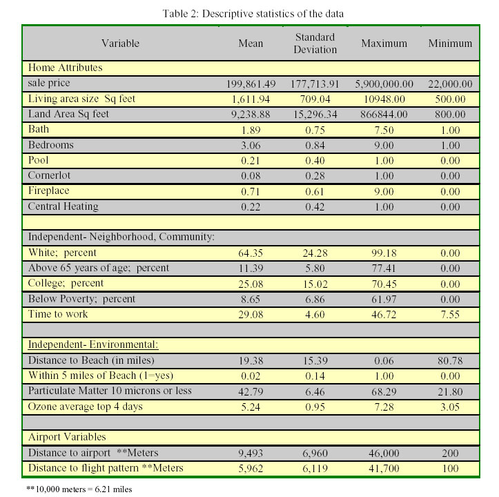
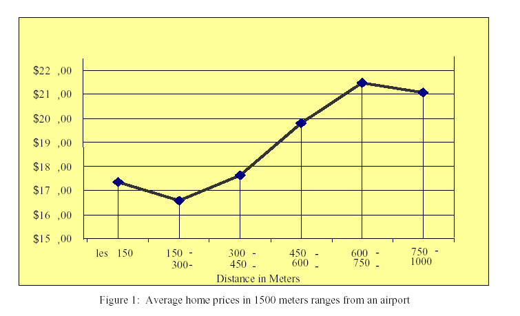
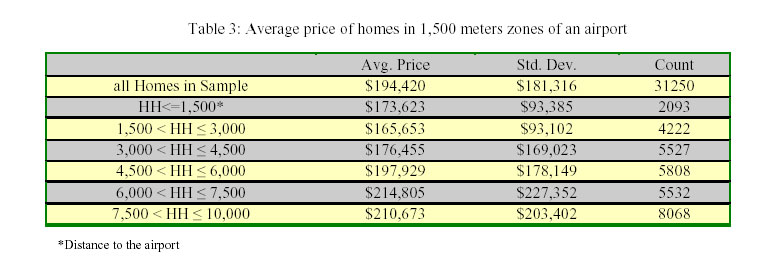
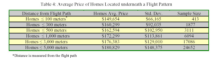
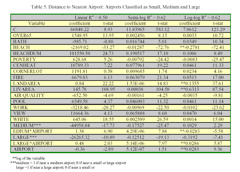
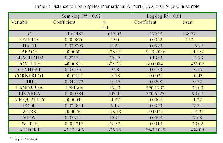
International Journal of Enviornmental Science and Technology, Vol. 1, No. 1, Spring 2004, pp.17-25 Airport noise and residential housing valuation in southern California: A hedonic pricing approach *M. Rahmatian and L. Cockerill Department of Economics, California State University, Fullerton, USA *Corresponding Author, E-mail: mrahmatian@fullerton.edu Code Number: st04003 Abstract A large and detailed data set is used to examine the influence of airports and airport light paths on housing prices. The results indicate that individuals consider airport proximity and airport flight patterns in their housing purchases. This shows that there exist two distinct measurable price gradients that distinguish large airports from small airports. In addition, homes located under the flight path of a large airport have a price gradient that is significantly larger than homes located under the flight path of a small airport. Key words: Hedonic property value, housing price evaluation, noise pollution Introduction A large airport generates an externality that must be shouldered by the residents that live within its influence. Noise, pollution, and increased traffic congestion are the most notable negative externalities associated with large airports. Instead of trying to directly measure the cost of an airport on resident well being this study uses differences in housing prices as a proxy estimate of the welfare loss associated with an airport in Southern California. A general price gradient representing the marginal implicit price of airport proximity is estimated using a cross section of 50,000 actual single-family home sales that took place in 1995. Distances to airports and airport flight paths have been assigned to every home in the sample. There are 23 airports included in the study, which generates enough spatial variation in the community variables to test the relative importance of airport proximity. The main assumption is that existing housing prices throughout Southern California have capitalized all the benefits and costs associated with living in a particular home. The results clearly show that individuals consider the presence of airports and airport flight patterns in their housing purchases (Freeman, 1992). A powerful and consistent price gradient with house price increasing with distance from an airport is observed. The results are relatively stable with respect to sample size and functional form. Furthermore, there is evidence to suggest that the price gradient changes slope with distance from an airport. That is, as distance increases the value of the average home increases but at a decreasing rate. It also appears that homeowners distinguish between large airports and small airports. Homes located underneath the flight pattern of a large airport have a price gradient that is steeper than homes located underneath the flight pattern of a small airport. This paper is organized as follows: Section two provides a brief review of the theoretical foundations of the hedonic housing value technique. Section three provides a description of the entire data set. Section four presents the empirical results using several different functional forms. Moreover, airport flight paths for both small and large airports are also examined. Finally, a summary and conclusion are offered in the last section. Theoretical model Underlying the ability to empirically elicit estimates of Willingness to Pay (WTP) for a latent characteristic is the assumption that there is a connection between observable private good purchases and the quantities or qualities of the latent variable under study. To derive a WTP function that lends itself to empirical techniques and allows for interpretable results, a structure must be imposed on the utility function. Freeman (1992) discusses the details of some of the imposed conditions that allow statistical estimation of the WTP function. Conditions such as weak seperability, weak complementarity, as well as treating the household's utility function as a production function are potential theoretical constructs that will yield interpretable formulations. Freeman explores the implications of each of these constructs and combinations of these constructs showing that the imposed conditions will allow for tractable formulations of the hedonic price equation, which subsequently permits derivation of the WTP function. The typical WTP function, i.e. inverse demand function for environmental quality (EQ) derived in most empirical studies is generated from the following underlying assumptions. Each household maximizes its utility subject to a budget constraint. Where: U = U (X, S, N, E) (1) X: the composite commodity It is assumed that there is a vast array of sizes and types of homes with many different neighborhood and environmental amenities. Individuals have information on all the different combinations and can choose from any location (Freeman, 1979). The market is assumed to be in equilibrium at a point in time and all consumers have chosen their utility maximizing array of housing characteristics. Given these assumptions the hedonic equation can be modeled as follows; Ph=a+b1s1+b2s2+...+bisi+c1n1+c2n2+...+ (2) cknk+d1q1+d2q2+...dgqg +...+dmqm S = (s1,s2,s3,....si) are structural characteristics; N=(n1,n2,n3..,nk) are neighborhood characteristics; Q=(q1,q2,q3,...qg...qm) are Environmental quality measures; The assumption of weak seperability in the utility function allows having a representation of the implicit price of EQ that is not a function of the level or prices of either structural or neighborhood characteristics. If we want to model that possibility then we need only impose a specific structure on the utility function to arrive at that kind of a result. Typically, empirical studies avoid that unnecessary complication and assume that the marginal rate of substitution within group characteristics is independent of each other. (Thayer, et al., 1998) The variable of interest is distance to the nearest airport. The data set has been organized so that distance to a small, medium or large airport can be distinguished. Homeowners should be more averse to living near a large airport as compared to living near a small or medium sized airport. An airport is considered large if annual passenger totals are greater than 100,000 per year. An airport is classified as medium if multi-engine jets land at the facility but passenger totals are less then 100,000 annually. Small airports do not accommodate passenger jets and are limited to small aircraft only. This study employs a slope shifter model in an attempt to estimate the price gradients for the three categories of airports using the following model. P (a)= b0 + b1a1 + b2D1 + b3D2 + (3) b4a1D1 + b5a1D2 + ∑ biai a1 = distance to the nearest airport Distance to the nearest airport and distance multiplied by the dummy variables are entered into the model. The net effect of distance is the sum of the two coefficients, which depends on the type of airport nearest to a household. The overview of the data set The data set includes 50,000 randomly selected observations from the Southern California Region. The sample was taken from a total population of nearly 106,000 recorded home sales that took place in 1995. The dependent variable for this study is actual home sale transaction price. The homes in the study are all single family dwellings. The independent data set includes variables that correspond to three types of attributes: structural, community, and environmental. A home's structure is described through such variables as square footage of living space, number of bathrooms, existence of a fireplace and ammenities such as a swimming pool. The community variables were derived from the 1990 census results. Variables such as percent of persons in census tract living below poverty level income, average time to work, percent of persons living in a particular tract with college degree, and percent white in tract were utilized for this study. Environmental variables included measurements of total average suspended particulate matter, level of ozone concentration, proximity to the ocean, and average visibility in miles. The variables of interest throughout this study will be distance to nearest airport and distance to nearest flight path. Table 1 provides a complete list of the variables utilized for this study.There are twenty-three airports included in the study area. The six largest airports ranked by passenger totals are: Los Angeles International, Orange County Airport, Ontario International, Burbank Airport, Palm Springs and the Long Beach Airport. The number of passenger boardings at the Los Angeles Airport is nearly three times the number of passenger boardings of all other airports in the study combined The average price of the 50,000 homes that were sold in 1995 was $199,861 with a standard deviation of $177,714. The average distance to the nearest airport is approxiametly 5.9 miles or 9,493 meters for all homes in the sample. The average distance to the nearest flight path is approximatetly 5,962 meters or 3.7 miles. The flight paths are imaginary lines that represent 10,000 meter extensions of an airport's runway configurations. The distance units meters is used for airport distance calculations throughout the entire study. The complete description of the data statistics are presented in Table 2. The harmful effects of multicollinearity among the independent variables is noted by researchers as the most troublesome of problems and should be carefully dealt with (Mendelson, 1985). Some multicollinearity is unavoidable among variables that describe the attributes of a home as well as the community attributes of the home's corresponding census tract. Since this study employs airport locations from several different geographical regions, spatial correlations as well as embedded biases of a single location should not be of serious concern (Beron, et al.,1998). The general methodology employed for the study was to pick a set of variables that were representative of the structural, community, and environmental attributes of a home but precluded the harmful effects of multicollinearity. Empirical Results Descriptive statistics of homes near airports The average price of homes in the sample tends to show a relationship between airport distance and home prices. Figure-1 shows a graph of the average price of all homes in 1,500-meter zones from an airport.Table-3 provides the actual average price of homes in 1,500-meter zones up to a distance of 10,000 meters. Table 3 provides the actual average price of homes in 1,500-meter zones up to a distance of 10,000 meters. Limited sensitivity analysis was then conducted to determine the robustness of the estimates. The difference in the price of a home located in the 7,500-10,000 meter range is on average worth $37,050 more then a home located within 1,500 meters of an airport. The difference in mean home prices for the two regions is statistically significant with a t-value of 8.6. Thus a 21% increase in the value of the home is realized if the homeowner is located an extra 6,000 to 7,500 meters from an airport. Table 4 provides a summary of the results on homes located near a flight path for all of Southern California. Homes located directly underneath a flight pattern or within 100 meters of a flight path had an average home price of $149,654. The average price of all homes located within 10,000 meters of an airport was $194,420 (from Table 3). The difference between the two averages is $51,766 and is significant with a t-value of 12.09. The difference between the average price of all homes within 10,000 meters of an airport and homes within 3,000 meters of a flight path is $18,037 and is statistically significant with a tvalue of 9.45. Distance to nearest airport: Airports classified as small, medium and large We initially used three functional forms, linear, semi-log, and log-linear, in an attempt to search for the best estimate of the marginal implicit price of airport influence. The three functional forms are widely used in empirical research of this kind because their coefficients lend themselves to interpretation (Palmquist, 1984), (Rahmatian, et al., 1992). The linear models provided coefficients that were similar to the semi-log and log-log models but the R2 was significantly smaller in several of the cases studied. Table 5 provides a summary of the three functional forms that were used in the initial model. Although the fit of the linear model is not as good as the semi-log and loglog formulations, the coefficients are very similar in sign and magnitude. The R2 of 0.5 for the linear model suggests that 50% of the variation in home prices can be accounted for by the explanatory variables. It is highly probable that a non-linear functional form will perform better than a linear form because people cannot costlessly repackage the characteristics of a home. Empirical studies such as (Beron, et al., 1998) and (Palmquist, 1984) reiterate this theoretical conjecture as well as many other studies employing the hedonic methodology (Rahmatian, et al., 1992) (Bartik, 1988).The interpretations of the explanatory variables that are not of primary focus provide some insight into whether the coefficients on AIRPORT (distance from airport) and the airport interaction terms are within reason. The linear model has predicted FIRE (existence of a fireplace) to be worth an additional $6,700 and a POOL to add $6500 to the value of the average home. If AIR QUALITY (annual average of TSP) increases by one milligram per cubic meter this has the effect of reducing home value by $650. A home with a VIEW can expect an increase in home value of about $11,600. For each mile from the BEACH (distance from beach in miles) the linear model estimates a decline in home price of $2,170. Modeling Los Angeles international airport (IAX) by itself Distance to LAX was assigned to every home in the sample. Semi-log and log-log regressions were run to estimate the implicit price of distance from LAX. The results of this experiment are displayed in Table 6. The coefficients on distance to LAX (AIRPORT) are negative and significant in both functional forms. The interpretation is that home prices fall as distance from LAX increases. Distance from LAX and the variable distance from the beach (BEACH) have a simple correlation of 0.81. If the LAX distance variable is removed, the coefficient on the BEACH variable becomes a larger negative number. If the variable BEACH is removed, the coefficient on distance from LAX increases substantially in the negative direction. We believe that Southern California's unique geography plays an important role in the results presented in Table 6. The general decline in housing prices distance inland increases outweighs the benefits of distance from LAX. Locating the distance at which airport effect is insignificant The coefficient on the variable AIRPORT in the models presented in the previous sections does not change with distance. The next step is to try to locate the distance at which the airport effect ceases to be a significant factor affecting the value of a home. Based on the results presented previously this study separates the sample into two groups, homes located near a small airport and homes located near a large airport. Separate regressions using dummy variables are applied to the two groups. The first experiment creates dummy variables representing homes located in 1,500-meter zones away from an airport. The control group is all homes located greater than 10,000 meters from an airport. The results suggest that the distance at which mean home prices are not significantly different from the control group is around 4,500 meters. It is interesting to note that the results for small and large airports are very similar. The semi-log results show the effects of small airports dying off but do not indicate a clear distance at which mean prices equalize. The semi-log model shows a slow dying off of the difference in home prices and does not cut off until around 15,000 meters and for the large airports suggest possibly more than one change in the price gradient. Airport flight paths for small and large airports Households are assumed to be more averse to living under an airport flight path than simply living near an airport. The next experiment uses a slope shifter model to test whether individuals are willing to pay a premium for distance from an airport if they are located under a flight path. A dummy variable is created that represents homes located under a flight path. Homes are designated to be under a flight path if they are within 1500 meters or approximately one mile from a flight path. A flight path is an imaginary line extended 10,000 meters in each direction of an airport's runway configuration. A slope shifter model of the following form is applied to both groups separately: P (a) = b0 + b1a1 + b2D1 + b4a1D1 + ∑ biai (4) Where a1 = distance to the nearest airport D1 = 0 if not in the flight path; = 1 if home in flight path ai = other explanatory variables The analysis of the sample of homes located near small airports results in the coefficients of 3.30E-06 and 0.0459 on the airport distance variable indicate that owners do take into consideration distance from a small airport. The coefficient on the flight path interactive term is not significant in the semi-log model, indicating that there does not exist a premium for homes located under small airport flight paths. The log-log model also indicates that homes do not consider flight paths. The sum of the control variable coefficient and the coefficient on the small airport interactive term (F-Path*AIRPORT) is nearly zero. The overall interpretation is that households do not consider living under flight paths of small airports to be significantly different then simply living near a small airport. Similarly, the analysis of the slope shifter model is applied to the set of homes designated close to a large airport. The coefficients on the interaction term in both the semi-log and log-log models are positive and significant, which suggests that households consider large airport flight paths in their home purchases. The cost of living under the flight path of a large airport is almost double the cost per meter of simple distance from a large airport. Conclusion and Summary This study provides estimates of the marginal implicit price of distance from large and small airports in Southern California. The problem with existing models is that they use small data sets and usually focus on estimating values in small homogeneous neighborhoods. This paper improves upon that by using a large data set to estimate housing prices. In addition this paper has included variables that will address the influence of time, seasonality and most importantly a location index. The marginal price of one additional meter from a large airport is worth nearly twice as much as an additional meter from a small airport. This study estimates that one additional meter from a large airport is worth approximately $1.23. The price per meter from a small airport is estimated to be between 65 and 77 cents. The marginal prices calculated are based on a mean distance from an airport of 9,500 meters. Homes located within 5,000 meters (3.10 miles) of a large airport have an average price that is estimated to be 4% to 10% lower then homes located greater than 5,000 meters from a large airport. Homes located within 5,000 meters of a small airport have a mean price that is 1.75% to 7.5% lower than homes outside the 5,000-meter perimeter. The marginal price per meter for homes located under the flight path of a large airport is not significantly different from the price per meter for homes near a small airport. The marginal price per meter for homes under the flight path of a large airport is approximately double that of homes located near a large airport but outside the flight path. The marginal prices are calculated at the mean of the airport distance variable. The estimates do not capture the possibility of a changing slope or changing elasticity as the mean of distance from an airport is reduced. Although marginal price is increasing with distance from an airport nonetheless this model does not control for changes in average home price and changes in the explanatory variables. Future research could focus on estimating a marginal price that changes with the mean of airport distance. Furthermore, the use of spatial techniques to handle spatial dependence of housing characteristics and sales prices would need to be explored. References
© 2004 Center for Environment and Energy Research and Studies (CEERS) The following images related to this document are available:Photo images[st04003t2.jpg] [st04003t5.jpg] [st04003t3.jpg] [st04003t6.jpg] [st04003t4.jpg] [st04003f1.jpg] [st04003t1.jpg] |
| |||||||||
