 |
| About Bioline | All Journals | Testimonials | Membership | News |
|
||||||
|
||||||
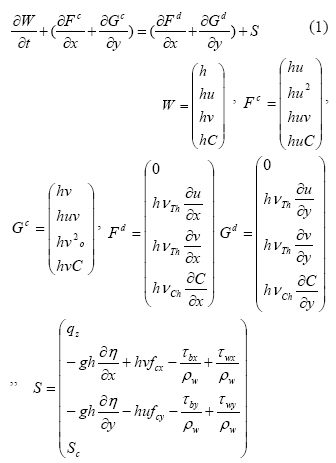
International Journal of Enviornmental Science and Technology, Vol. 1, No. 1, Spring 2004, pp.39-44 Numerical modeling of Persian Gulf salinity variations due to tidal effects *S.R. Sabbagh Yazdi Department of Civil Engineering, Khaje Nasir Toosi University of Technology, Tehran, Iran *E-mail: syazdi@kntu.ac.ir Code Number: st04005 Abstract Numerical modeling of salinity changes in marine environment of Persian Gulf is investigated in this paper. Computer simulation of the problem is performed by the solution of a convection-diffusion equation for salinity concentration coupled with the hydrodynamics equations. The hydrodynamic equations consist of shallow water equations of continuity and motion in horizontal plane. The effects of rain and evaporations are considered in the continuity equation and the effects of bed slope and friction, as well as the Coriolis effects are considered in two equations of motion. The cell vertex finite volume method is applied for solving the governing equations on triangular unstructured meshes. Using unstructured meshes provides great flexibility for modeling the flow problems in arbitrary and complex geometries, such as Persian Gulf domain. The results of evaporation and Coriolis effects, as well as imposing river and tidal boundary conditions to the hydrodynamic model of Persian Gulf (considering variable topology rough bed) are compared with predictions of Admiralty Tide Table, which are obtained from the harmonic analysis. The performance of the developed computer model is demonstrated by simulation of salinity changes due to inflow effects and diffusion effects as well as computed currents. Key words: Persian Gulf, modeling, salinity, tidal effects, computer simulation Introduction The computer simulation of complicated marine environment problems have become one of the interesting areas of the research works by the availability of the high performance computers. The control over properties and behavior of fluid flow and relative parameters of the inclusive soluble materials are the advantagess offered by numerical simulation of fluid flow problems. Hence, developing efficient and accurate numerical algorithms suitable for the complex flow domain has become a challenging task. Recent advances in development of efficient numerical modeling techniques encourage the application of advanced modeling algorithms for solution of fluid flow engineering and environmental problems. Governing equations The convection- equation of pollution phenomena, which is formed by both transport and diffusion terms, is applied to model the salinity variations due to the inflow concentrations and diffusion effects as well as transport by computed currents. The depth averaged (shallow water) equations are chosen as the governing equation of the flow in the Persian Gulf. The governing equations are written in vector form as follows:
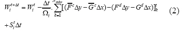
Where, W represents the conserved variables using h flow depth, u and v the horizontal components of velocity, and C soluble material (salinity concentration). Gc and Fc are vectors of convective fluxes, while, Gd and Fd are vectors of diffusive fluxes of W in x and y directions, respectively. The vector S contains the source and sinks terms of the governing equations (Vreugdenhil, 1994.) Using above equations, the currents in Persian Gulf are computed considering qz the evaporation from the water surface, surface and bed slopes η = h + zb , global bed friction stresses However, the boundary conditions of river inflow and tidal effects in Hormoz strait play important roles in forming time-dependent currents. Similarly, the percentage of the concentrations at the flow boundaries as well as the amount entering from the point sources affect the computed distribution of the soluble material in the flow field. Numerical formulations The equations are explicitly solved using Cell Vertex Finite Volume Method on triangular unstructured meshes. Application of unstructured mesh facilitates considering the effects of geometrical irregularities of coasts and islands. The governing equations are discretized by the application of cell vertex (overlapping) scheme of the finite volume method. This method ends up with the following formulation. (Jameson, et al., 1986).
Where Wi represents conserved variables at the center of control volume Ωi. The residual term:
consist of convective and diffusive part. In smooth parts of the flow domain, where there is no strong gradient of velocity components, the convective part of the residual term is dominated. Since, in the explicit computation of convective dominated flow there is no mechanism to damp out the numerical oscillations, it is necessary to apply numerical techniques to overcome instabilities with minimum accuracy degradation. In present work, the artificial dissipation terms suitable for the unstructured meshes are used to stabilize the numerical solution procedure. In order to damp unwanted numerical oscillations, a fourth order artificial dissipation term,
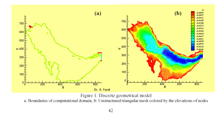
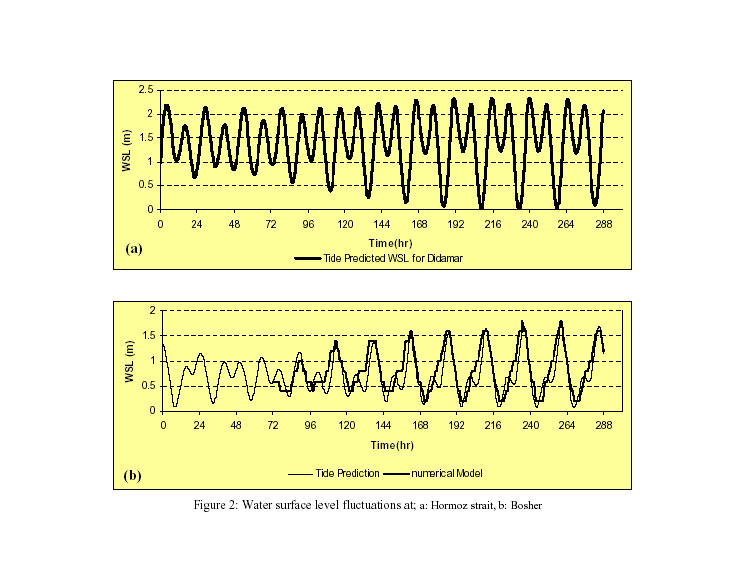
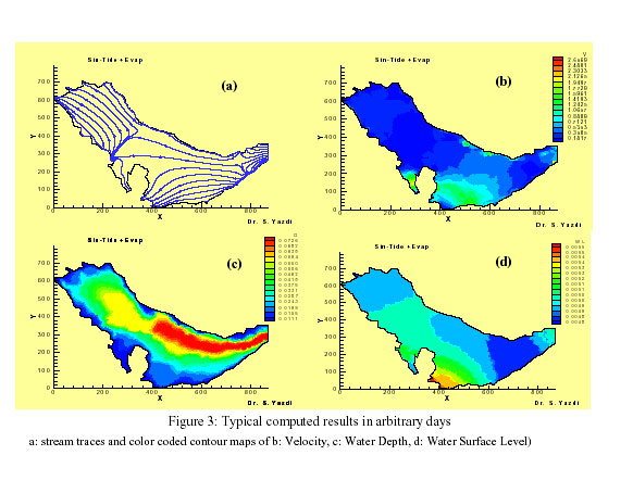
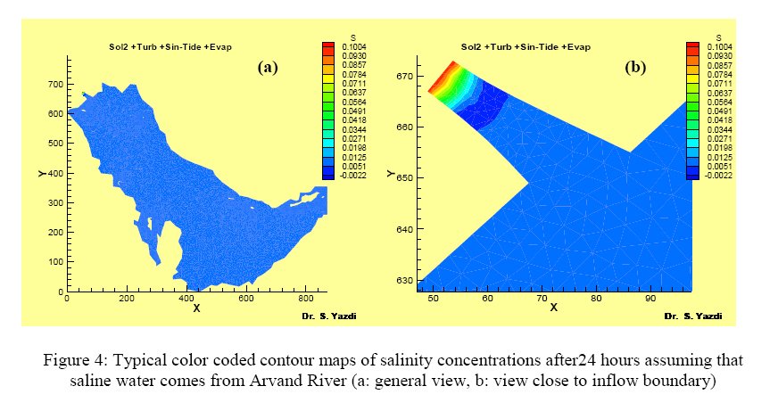
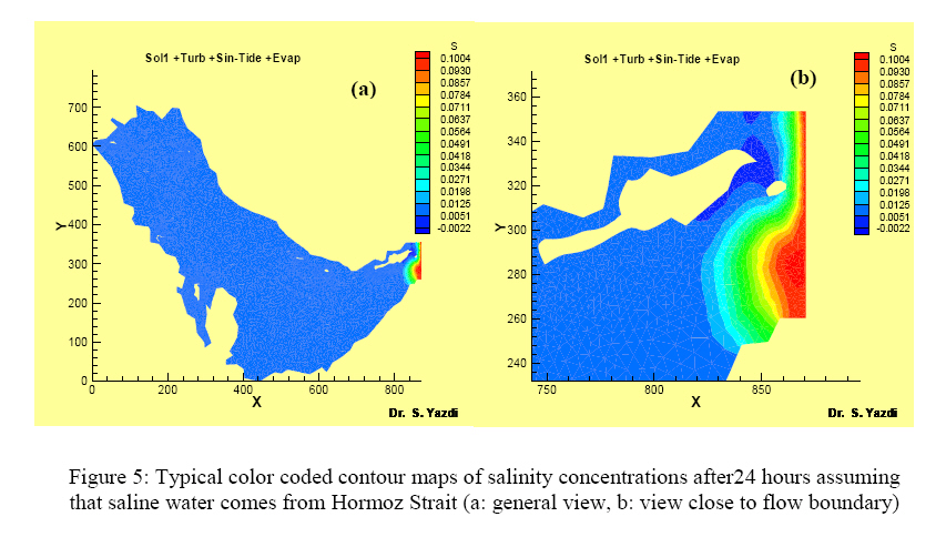
Δt is the minimum time step of the domain (proportional to the minimum mesh spacing). In present study, a three-stage Runge-Kutta scheme is used for stabilizing the explicit time stepping process by damping high frequency errors (Jameson, et al., 1981). In the above equation, the quantities W at each node is modified at every time step by adding a residual term which is computed using the quantities W at the edges of the control volume Ωi. Hence, the edges are referred to all over the computation procedure. Therefore, it would be convenient to use the edge-base data structure for definition of unstructured meshes. Using the edge-base computational algorithm reduces the number of addressing to the memory and provides up to 50% saving in computational CPU time consumption. Hence, the edge-base algorithm and data structure improves the efficiency shortcoming of the unstructured mesh data processing (Sabbagh Yazdi, 2001) Boundary conditions Two types of boundary conditions are applied in this work: flow and solid wall boundary conditions. Flow boundaries The tidal flow boundary condition is considered by imposing of water surface level fluctuations at Hormoz strait. In this case, the velocity components at Hormoz strait are extrapolated from the computational domain. The fluctuations of water surface elevation are from tidal predictions at Didamar Island, which can be obtained by application of the calibrated constants of the harmonic analysis provided by Admiralty Tide Tables (Admiralty Tide Tables, British Admiralty, 1964) for any arbitrary period of time. At the tidal flow boundary, the inflow value for the concentration variable C from the Indian Ocean may be imposed when the computed velocity is toward the flow domain. The river inflow is imposed whenever the inside domain water surface level is less than the water level at the flow boundary. The monthly averaged inflow rate of the Arvand River is suitable to apply for the computation of inflow velocity. In such a case, water surface elevation at river boundary has to be extrapolated from the computational domain. Otherwise, all the flow parameters have to be extrapolated. The value of inflow concentration variable C from the river can be imposed at river flow boundary when the inflow velocity is imposed. Wall boundaries The dry parts at coastal zones and islands boundaries are the flow domain limits. At these boundaries the component of the velocities normal are set to zero. Since the application of wet and dry conditions at wall boundaries require grid refinement all over the wall boundaries, a fine margin along the wall boundaries are ignored. Therefore tangential computed velocities are kept using free slip condition at wall boundaries. Although small water depth in coastal zones get rise to the global bed shear stresses and reduce the computed velocities, tangential velocity reduction coefficient may be used to model the effect of wall boundaries. Therefore, at this wall boundary type a rough wall boundary type is introduced (Sabbagh Yazdi and Mohamad Zadeh, 2003). However, no velocity reduction coefficient should be used at the wall boundaries, which intersect flow boundaries. Therefore, another type of wall boundary type introduced as fully free slip wall type. At wall boundaries, which are set to this type, only the component of velocity vector normal to the solid boundary edges are set to zero. (Sabbagh Yazdi, 1997). Application of free slip velocity condition provides considerable savings on computational efforts, since there is no need to reduce mesh spacing in the vicinity of the wall boundaries. Geometry modeling Persian Gulf flow domain is modeled in two stages. In the first stage, horizontal geometry of the problem is modeled by definition of 175 boundary curves, which represent coastal boundaries and eight major islands. Then, the flow domain is discretized using unstructured mesh generated by Deluaney Triangulation Technique (Weatherill, 1996). The mesh was which contains 7995 nodes, 14938 elements, and 22940 edges, is refined at flow boundaries. In the second stage, the bed elevation of the flow domain is digitized at a number of points along some contour lines. Then, the bed elevation is set for the every node of the mesh by interpolation of the elevations of surrounding digitized points. Therefore, the geometry of a three dimensional surface is modeled in digital environment. The two dimensional boundaries if the computational domain inside which is filled with triangular elements is plotted in figure 1 a. The unstructured triangular mesh, which is converted to a three dimensional surface as the flow domain bed is demonstrated in figure 1-b. In following sections, the numerical simulation of salinity distribution in Persian Gulf is presented after evaluation of the accuracy of the developed hydrodynamic model. Hydrodynamic model The described hydrodynamic model, which solves depth-averaged equations of continuity and motions, is used to compute flow patterns in Persian Gulf. In order to verify the quality of the results, the tidal fluctuations at Didamar Island, obtained from Admiralty Tide Table for the period of 12 days from December 2003 the 1st (Figure 2-a), are imposed at Hormoz Strait (the east end of the flow domain). The inflow from the Arvand River (located at the border line between Iran and Iraq) is imposed at the end the estuary located at the south west of the flow domain. Considering the evaporations from the water surface and Coriolis effects, the flow patterns are formed due to the bed surface geometry and roughness. In Figure 2-b, the water surface elevation computed by the hydrodynamic model (thick line) is compared with the predictions of the Admiralty Tide Table (thin line) at Bosher Port, which is located at the north part of the Persian Gulf. Since still water is consider at the start of the computations, there is a few days warm up period and then the results of the hydrodynamic model follow the Tide Table predictions. A few samples of numerical results, which present computed water surface elevation and flow patterns are shown in Figures 3. These computed results present stream traces (a) and color coded contour maps of velocity magnitude (b), water depth (c), and water surface level (d) in an arbitrary days Salinity distribution modeling The model efficiency of the developed numerical algorithm is utilized to model the salinity distribution in Persian Gulf. Considering the fact that the percentage of salinity concentration in flow domain is different from the inflow currents entering from the Arvand River and Hormoz Strait, the behavior of the computer model is investigated for a short period of time. The concentrations distribute due to the diffusivity and currents. Figures 4 and 5 present patterns of the salinity concentrations close to the flow boundaries of Persian Gulf. It is interesting to see that the salinity concentrations have different characteristics in various part of the Persian Gulf. This is due to formation of various velocity fields in different part of the flow domain. Conclusions Solving the depth averaged equations of continuity and motions unstructured triangular mesh considering the bed elevation develops a hydrodynamic model. The model is able to consider fluctuations at tidal flow boundary, inflow from rivers, evaporations and Coriolis effects, bed surface geometry and roughness. The agreements between predictions of Admiralty Tide Table and flow patterns computed by hydrodynamic model encouraged coupling a convection diffusion equation to model variations of salinity concentration in the flow field, and therefore, the transport and diffusion of concentration is successfully simulated. The results of numerical modeling of the salinity variations showed the pronounced effect of the incoming flow from the Hormoz Strait. Although this fact matches with the general expected fact, the advantage of numerical modeling is to provide fine details of salinity concentrations in computational flow domain. Acknowledgement This work is financially supported by KNT University of Technology. References
© 2004 Center for Environment and Energy Research and Studies (CEERS) The following images related to this document are available:Photo images[st04005f2.jpg] [st04005f5.jpg] [st04005f3.jpg] [st04005f1.jpg] [st04005f4.jpg] |
| |||||||||
