 |
| About Bioline | All Journals | Testimonials | Membership | News |
|
||||||
|
||||||
International Journal of Enviornmental Science and Technology, Vol. 1, No. 1, Summer 2004, pp. 141-150 Modeling contaminant transport in soil column and ground water pollution control *S. A. Mirbagheri Department of Civil Engineering, Shiraz University, Shiraz, Iran *E-mail: www.Dr.mirbagheri.com Code Number: st04018 Abstract A mathematical and computer model for the transport and transformation of solute contaminants through a soil column from the surface to the groundwater is presented. The model simulates selenium species such as selenate, selenite, and selenomethionine as well as pesticides and nitrogen. This model is based on the mass balance equation including convective transport, dispersive transport, surface adsorption, oxidation and reduction, volatilization, chemical and biological transformation. The governing equations are solved numerically by the method of implicit finite difference. The simulation results are in good agreement with measured values. The major finding in the present study indicates that as the time of simulation increases, the concentration of different selenium species approaches the measured values. Key words: Mathematical, computer, model, contaminant transport, selenium species, groundwater pollution Introduction Mathematical modeling is an accepted scientific practice, providing the mechanism for comprehensively integrating basic processes and describing a system beyond what can be accomplished using subjective human judgements. It is possible to construct models that better represent the natural system, and to use these models in an objective manner to guide both our future research efforts and current management practices. Recent years have seen a variety of approaches to description of water and solute movement in soils field. A number of new models have been proposed in response to recently collected field data on solute leaching patterns. Many of them have been produced as the result of research into basic physics and chemistry of salt, nitrogen, pesticide transport and transformation in agricultural soils. Leachates from sanitary landfills are also recognized as important groundwater pollutants. The contaminants are released from the refuse to the passing water by physical, chemical, and microbial processes and percolate through the unsaturated environment, polluting the groundwater with organic and inorganic matter. The modeling of contaminant transport hinges on an understanding of the mechanisms of mass release from the solid to the liquid phase, and contaminant decay. These mechanisms are influenced by such factors as climatic conditions, type of waste, site geohydrologic conditions, and chemical reactions as well as microbial decomposition of organic matter. Modeling of different kinds of contaminant was studied by several researchers, Ahlrichs and Hossner (1987), Alemi, et al., (1988), shifang (1991), Alemi, et al., (1991), Hutson and Wagenet (1989), Copoulos, et al., (1986), Thompson and Frankenberger (1990), Tanji and Mehran (1979), and Hooshmand (1992). The objective of this paper is to addresses the spatial and temporal distribution of contaminant concentrations in soil column. Also, to develop a dynamic simulation model, which approximates contaminant concentrations in groundwater systems under unsteady water flow conditions where microbial activities and plant growth were present. The work has been done in Shiraz University in 1997. Mathematical Model The flow and the corresponding moisture content and the concentration of a contaminant are considered here in as continuous functions of both space and time. This model considers a variety of processes that occur in the plant root zone as well as leaching to the ground water, including transient fluxes of water and contaminants, alternating periods of rainfall, irrigation and evapotranspiration, under variable soil conditions with depth. Water flow model Water flow is calculated using a finitedifference solution to the soil-water flow equation
Where h is a soil water pressure head (mm), θ is volumetric water content (m3m-3), t is time (day), H is hydraulic head (h + z), z is soil depth, K is hydraulic conductivity (mm day –1),
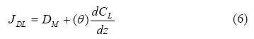
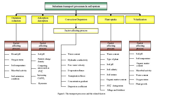
Where hi =a[2b /(1+2b)]−b and θi =2bθ s /(1 +2b)is the point hi, qi of intersection of the two curves, θ s is water content at saturation, a and b are constant. The two curves are exponential and prabolic for dry and saturated soil respectively. Similarly the equations for hydraulic conductivity can be derived as a function of soil water pressure head. When soil water pressure head is greater than hi the following equation is used to calculate hydraulic conductivity: K (θ)=Ks (θ /θ s )2b+2+p (3) Where Ks is hydraulic conductivity at saturation water content (θ s ) , and P is Pore water interaction parameter. When soil pressure head is less than hi the equation for the calculation of hydraulic conductivity is: K =Ks (a / h)2 +(2+P)/ b (4) Solving equation (1) using finite difference techniques provides estimated values of h at each depth node used in the differencing equation. Water contents are calculated using equation (2). Water flux densities (q) are calculated over each depth interval using Darcy’s equation Contaminant transport model The bulk motion of the fluid, and controls contaminant transport through the soil column by molecular diffusion and mechanical dispersion. Mixing due to molecular diffusion is negligible compared to that caused by dispersion. At the same time generation of loss of mass takes place due to adsorption and adsorption, and the biokinetics of the mass dissolved or suspended in the moving water. In this study selenium, nitrogen and pesticide were modeled. Figure 1 shows some of the selenium transport and transformation processes and the factors affecting each of the processes. In general for steady–state water flow condition the transport terms for selenium are: Js =J DL +JCL (5) Where Js is total selenium flux
Where CL is concentration in the liquid phase and DM(θ ) is the molecular diffusion coefficient. The value of DM (θ ) can be estimated (Kemper and Van Schaik, 1966) as:
Where DOL is the diffusion coefficient in a pure liquid phase and a and b are emprical constants reported by Olsen and Kemper (1981) to be approximately b = 10 and 0.005 < a < 0,01 the convective flux of selenium can be represented as:
Where q is the water flux, and Dh (q) is the hydrodynamic dispersion coefficient that describes mixing between large and small pore as the result of local variations in mean water flow velocity. Combining the molecular diffusion coefficient and hydrodynamic dispersion coefficient as: D (θ , q ) = DM (θ ) + qDh ( ) (9) Where D (θ , q ) is the apparent diffusion coefficient (cm-2 day-1). Substituting equations 6, 8 and 9 into equation 5 the overall selenium flux is given as:
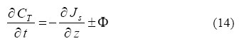
Partitioning selenium between sorbed and solution phases, according to Alemi (1991), adsorption of selenium are assumed taken to be nonlinear equilibrium process described by: Cs = CsK n (11) Where Cs is the concentration of selenium absorbed on the soil ( α mole K-1), Ks is the adsorption coefficient for selenium (L Kg-1), C is the concentration of selenium in the soil solution ( α mole L-1), n is the nonlinear equilibrium adsorption reaction exponent for selenium. The total amount of selenium (CT) contained in the solution and adsorbed phases in a soil volume of one liter are: CT = ρ Cs +θ Cl (12) Where ρ is the soil bulk density (g cm-3). Substituting equation (11) for Cs in equation (12) one can get the convection-dispersion equation: CT = Cl + (θ + ρ Ks ) (13) Selenium transports in soil system occur under nonsteady (transient) water flow condition. The water content (θ ) and water flux (q) both vary with depth and time. Using continuity relationships of mass over space and time gives:
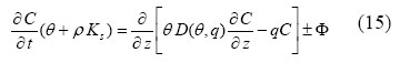
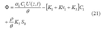
Where CT the total selenium concentration in sorbed and solution is phases and φ represents all sources or sinks of selenium. Substituting equation (8) and (13) into (14) gives general one-dimensional transport equations for selenium transport:
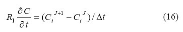
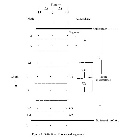
Where C is concentration of all selenium species in soil solution, and φ indicates all possible sources or sinks term. The sources and sinks of selenium in soil system under the field condition result from the following processes: A. Transformation of selenate to selenite and selenite to elemental selenium. B. Volatilization of selenate, selenite and selenomethionine to Dimethyl Selenide (CH3) 2 Se. C. Imobilization and mineralization of selenate and selenite to organic selenium. D. Decomposition of organic selenium to selenomethionine. E. Plants uptake of selenate, selenite and selenomethionine. Equation 15 is in general form, similar equation can be written for different nitrogen and pesticides species in soil column. Solution procedure Prediction of the concentration of selenate, selenite and selenomethionine in all phases (liquid, sorbed, gas) as well as leaching losses at any depth for all time levels requires simultaneous solution of equations for all selenium species. The equations are solved numerically using an implicitly finite difference scheme and crank-nikolson approximation. Using Figure 2 for the nodes and segments as well as time interval; the first term in equation (15) is evaluated at node i and time l j+1/ 2 and is differenced as: C= C1
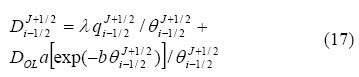
The second term in equation (15) is a diffusion and dispersion term. D (, q) for the interval between nodes i-1 and i is differenced as:
Where
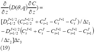
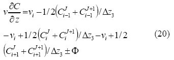
The convection term in equation (15) is differenced as:
Multiplying out and collecting the unknown CiJ +1 terms on the left-hand side and the know CJ terms on the right-hand side, the general form of equation as:
Where Di considers all the sources and sinks in equation (16). For example the sources and sinks term for equation (16) are:
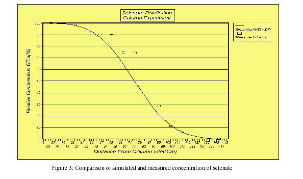
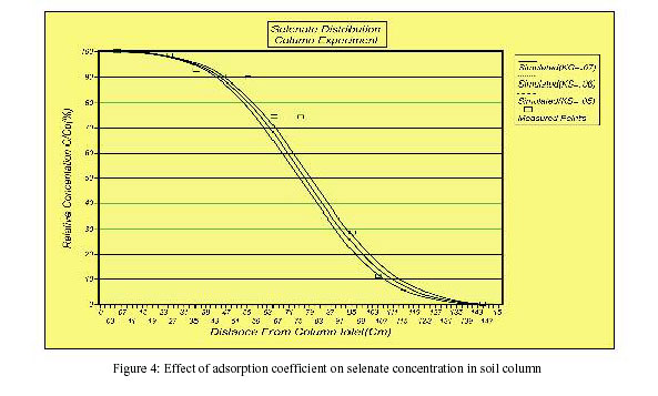
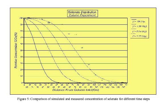
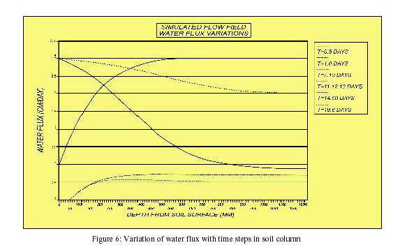
The finite difference forms are written similarly for all other equations for each node from 2 to K-1 where K is the lowest node in the profile. This set of equations, then is solved for defined boundary conditions using the Thomas tridiagonal matrix algorithm. Upper and lower boundary conditions The boundary conditions for solute and water flux are not always the same algebraic sign within each time interval as water can evaporate from the soil surface while salt accumulates. The upper boundary condition for selenium needs to be defined to represent zero flux, infiltration the value of C1 J =Cw and surface evaporation C1 J = 0, The lower boundary condition for selenium needs to be defined for zero flux, water table and unit hydraulic gradient. For zero flux Results The model was applied to simulate contaminants such as selenium, pesticide and nitrogen in soil column under steady state and transient water flow conditions. The soil column was assumed to be unsaturated under both conditions. For the simulation of selenium species such as selenate, selenite and selenomethionine. The data collected by (Alemi, et al., 1991) was usded. In their study under steady-state water flow conditions, 150 to 210 ml of influent solution containing 19.23 mol L-1 of Se in the form of sodium selenate, sodium selenite and selenomethionine were applied to the column. The water flow through the soil volume was 1.44 cm day –1 in cm of soil column. The experiment was run for 2.77 days. At the end of each run the concentration of different Se species were measured in soil profile. The data from the results of the experiment was used to run model. The time and distance interval for running the model were 0.02 day and 0.25 cm respectively. The results indicate that transport model adequately simulates the measured quantities as shown in Figure 3. The simulation results for total time from 0.68 day to 2.77 days indicate that as the time increases the influent concentration approaches the inflow, which is comparable with measured values as shown in Figure 4. The sensitivity analysis of the model to some parameter at steady state water flow condition shows that the model is very sensitive to the adsorption coefficient, KS, such that by increasing the KS from 0.05 to 0.07 liter Kg-1, the simulation results get closer to measured values as shown in Figure 5. The model also simulates the concentration of other selenium species and contaminants, (Mirbagheri and Tanji, 1995). LEACHM was used for the simulation of water content and water flux. The texture of the soil profile assumed to be uniform and composed of 28 percent clay, 30 percent silt and 42 percent sand. The hydraulic conductivity of soil was assumed to be 11.4 md-1 with 55 percent saturation condition. The simulation results for the water flow model are shown in Figure 6. The curves in Figure 6 show an exponential and parabolic relations exits in soil profile under saturation and unsaturation soil conditions. Discussion and Conclusion One-dimentional water Flow and contaminant transport model was applied to simulate selenate, selenite and selenomethionine in soil column. The model predicts the concentration of different contaminant in goroundwater. The simulation results indicate as the total time from the beginning to the end of simulation increases, the concentration of selenate, selenite and selenometionine approaches the measured values, as indicated in the results section the model is sensitive to adsorption coefficient, Ks. as Ks increases the relative concentration of selenate increases. The results also shows the variation of water flux with times steps in soil column, as the time increases from 0.5 days to about 20 days the water flow approaches the steady state. LEACHM, which is the Leaching Estimation and Chemical Model, was used for the simulation of water flux and hydraulic conductivity of soil used in the study area. The model was very useful tool for the estimation of water content. The model can be used for the prediction of water pollution in groundwater systems. Notation θ = Volumetric water content References
© 2004 Center for Environment and Energy Research and Studies (CEERS) The following images related to this document are available:Photo images[st04018f4.jpg] [st04018f1.jpg] [st04018f5.jpg] [st04018f3.jpg] [st04018f6.jpg] [st04018f2.jpg] |
| |||||||||

 is differential water capacity, and u is a sink term representing water lost by transpiration (absorption of water by plant). Functions which characterized relationships between K −θ − h described in LEACHM (Hutson and Wagenet, 1989) are used. There is a two-part function that described the general shape of θ (h) relationships (Hutson and Cass, 1987),
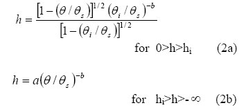