International Journal of Environment Science and Technology Center for Environment and Energy Research and Studies (CEERS) ISSN: 1735-1472 EISSN: 1735-2630 Vol. 2, Num. 1, 2005-2006, pp. 13-26

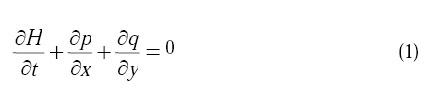
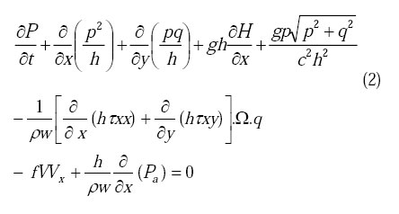
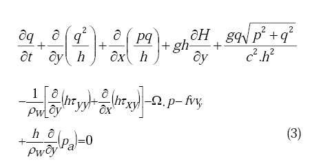
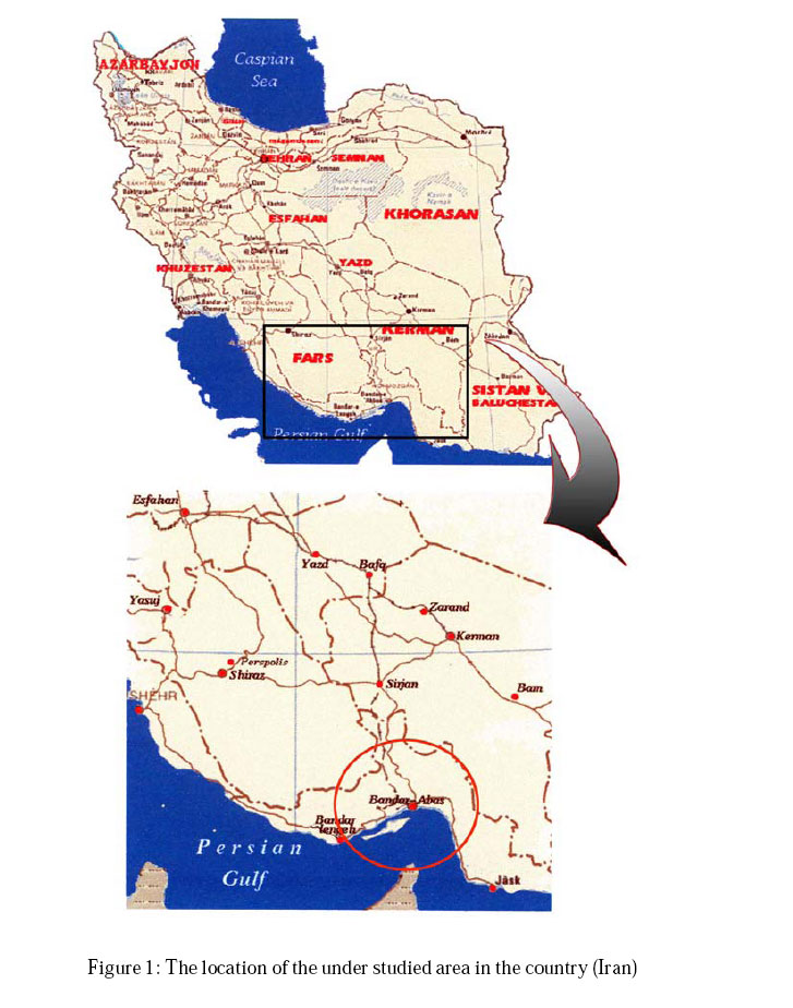
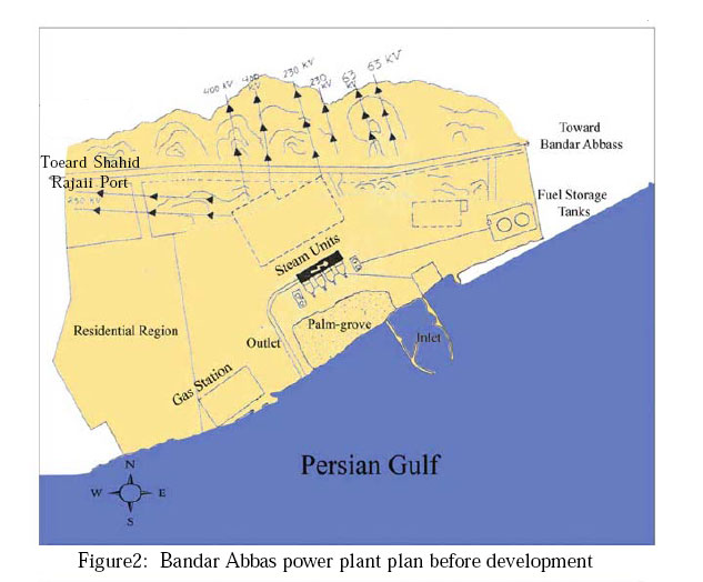
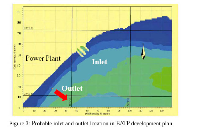
International Journal of Enviornmental Science and Technology, Vol. 2, No. 1, Spring, 2005, pp. 13-26

Modeling of thermal pollution in coastal area and its economical and environmental assessment

^1*M. Abbaspour , ²A. H. Javid, ²P. Moghimi and ³K. Kayhan

¹Department of Mechanical Engineering, Sharif University of Technology, Tehran, Iran
²Department of Environmental Engineering, Graduate School of the Environment and Energy, Science and Research Campus, Islamic Azad University, Tehran, Iran
³Technical Manager of Danish Hydraulic Institute (DHI) in Iran, Tehran, Iran
*Corresponding Author, E-mail: m-abbaspoor@jamejam.net

Code Number: st05003

Abstract

The Persian Gulf is one of the aquatic ecosystems which has recently faced with different pollutions. Cooling water discharges due to various industries such as power plants can cause important disorders on present ecosystem balance because of its high temperature. Obviously, due to thermal pollution, a great number of aquatic creatures face with a new situation that they can not tolerate. Thermal pollution leads to their migration, creates a potential for new coming species which in turn can thoroughly change the marine ecosystem feature. The other impacts of this phenomenon are: disorders in reproduction, nourishment and other biological habits. In this research, thermal pollution due to Bandar Abbas Thermal Power Plant (BATP) development plan was modeled using MIKE21 software. In order to avoid a decrease on the power plant efficiency in development plan, the distance between inlet and outlet was determined by comparing the results of different scenarios and economical aspects. After determining the distance between inlet and outlet, the water temperature in the coastal area was compared with standards of Iranian Department of the Environment (DOE). The model results represent that the water temperature, in Bandar Abbas coastal area, exceeds than the permissible limit (3 °C) in a distance equal to 200 m. far from the discharging location, and in order to reduce its harmful impacts, some suggestions are made to reduce the associated thermal pollution.

Key words: Power plant, thermal pollution, modeling, Persian Gulf, MIKE21

Introduction

Chemical industries, fossil fuel and nuclear power plants use lots of water for cooling purposes and return this water to environment at a higher temperature. The hot water interferes with the natural conditions in the sea, lake or river affecting aquatic life. This is thermal pollution when heat acts as a pollutant (Kummar and Kakrani, 2000). Hitherto, the largest quantities of heat have been due to cooling water discharge from power plants (Zahid and Mohammadi, 2000). In the southern part of Iran, cooling water from Boushehr, Kish and Bandar Abbas power plants is directly discharged to the coastal area of Persian Gulf which has harmful consequences on marine ecosystem. In this research, thermal pollution distribution due to Bandar Abbas Power plant development plan in coastal area was modeled by software and the water temperature increase was compared with standards of Iranian Department of the Environment (DOE), and finally some suggestion was made to reduce the associated thermal pollution. The location of the understudy area in the country is illustrated in Figure 1. Bandar Abbas Steam Power Plant has four steam units, and the power generation of each of them equals to 320 MW. It is located at (56^o 7' E, 27^o 8' N) near the coast of Persian Gulf (Samadi, 1997). The required water for the condenser, cooling towers and water desalination units is 50 m³/s which is taken from the Gulf. Two adjacent concrete channels discharge the sewage into the Gulf (Figure 2).In the power plant development plan, it is decided that two steam units be added (the power generation of each of them equals to 325 MW). Therefore the total discharge for the power plant reaches to 75 m³/s, and three adjacent concrete channels will discharge the whole sewage in a location that the hot water will not affect the efficiency of the power plant more than specific amount (Figure 3).

Hydrodynamic equations

The conservation of mass and momentum integrated over the vertical are used in the hydrodynamic model to describe the flow and water level variations (MIKE21, 2003):

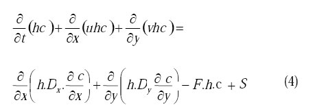
The following symbols are used in the equations:
h (x, y, t): water depth (m)
H (x, y, t): surface elevation (m)
p, q (x, y, t): flux densities in x and y directions (m³/
(s.m))
c (x, y): Chezy resistance (m^1/2 /s)
g : acceleration due to gravity (m/s²)
f (v) : wind friction factor
v ,v_x , v_y (x,y,t) : wind speed and components in x
and y direction (m/s)
Ω (x, y): coriolis parameter (s^-1)
P_a : atmospheric pressure (Kg/m.s²)
ρw: density of water (kg/m³)
x,y : space coordinates (m)
t : time (s)

τ _yy, τ _xy, τ _xx: components of effective shear stress (N/m²)

Advection dispersion equation

The advection dispersion equation is solved for dissolved or suspended substances in two dimensions. It is in fact the mass-conservation equation. Discharge quantities and compound concentrations at source and sink points are included together with a decay rate (MIKE 21 Environmental Hydraulics Advection –Dispersion Module, scientific Documentation, 2003).

The following symbols are used in the equation:

c: compound concentration (arbitrary units)
u, v: horizontal velocity components in x, y directions
(m/s)
h: water depth (m)
D_x, D_y: dispersion coefficients in the x, y directions
(m²/s)
F: linear decay coefficient (sec ^-1)
S = Q_{s .}(c_s - c)
Q_s : source/sink discharge (m³/s/m²)
c_s: concentration of compound in the source/sink discharge (arbitrary units)
Information on u,v and h at each time step is provided by the hydrodynamic module.

The most common use for a heat dissipating substance is that of modeling power plant cooling water recirculation .Here the advected and dispersed component is heat (or rather temperature).The heat dissipation follows a prescribed function where the decay factor F may take the following form:

F = 0.2388/(ρ.Cp.h).[(4.6 − 0.09(T_ref +T_e ) + 4.06w).exp(0.033(T_ref + T_e ))](5)

Which is suitable for heat dissipation to the atmosphere. (MIKE21, Environmental Hydraulics Advection–Dispersion Module, Scientific Documentation, 2003).
Where:

w: wind speed (m/s)
T_ref: the reference temperature (°C)
T_e : excess temperature (°C)
ρ : density of water (kg/m³)
Cp: specific heat (cal/kg °C)

Near shore spectral wave equations

These basic equations in the model are derived from the conservation equation for the spectral wave action density; and are as the forms bellow (MIKE 21 Nearshore Spectral Wind-Wave Module, Scientific Documentation, 2003):

Where:
m₀ (x, y, θ):Zeroth moment of the action spectrum
(m²)
m₁ (x, y,θ): First moment of the action spectrum
(m² /s)
c_gy, c_gx:Components in the x and y direction of the
group velocity (c_g) , (m/s)
_cθ: propagation speed representing the change of action in the θ direction (m/s)
θ : direction of the wave propagation (degree)
S₀, S₁: source terms (m², m²/s)
The moments m _n(θ) are defined

Where ω is the absolute frequency (s^-1), and A is the spectral wave action density (m²/s).

The propagation speed c_gx,c_gy and c_θ are obtained using linear wave theory.

The left hand side of the basic equations (6) takes into account the effect of refraction and shoaling .The source terms S₀ and S₁ take into account the effect of local wind generation and energy dissipation due to bottom friction and wave breaking. The effects on current on these phenomena are included.

Numerical solution specifications for hydrodynamic equations

There is used of a so-called Alternating Direction Implicit (ADI) technique to integrate the equations for mass and momentum conservation in the spacetime domain. The equation matrices that result for each individual grid line are resolved by a Double Sweep (DS) algorithm. The numerical solution has the following properties (MIKE21 Coastal Hydraulics and Oceanography, Hydrodynamic Module, Scientific Documentation, 2003):

• Zero numerical mass and momentum falsification and negligible numerical energy falsification, over the range of practical applications, through centering of all difference terms and dominant coefficients, achieved without resort to iteration.
• Second-to third-order accurate convective momentum terms, i.e.” Second-and third-order” respectively in terms of the discretization error in a Taylor series expansion.
• A well-conditioned solution algorithm providing accurate, reliable and fast operation.

Numerical solution specifications for advection dispersion equation

It is used of a third order finite difference scheme QUICKEST which in many ways has very fine qualities .It avoids the wiggle instability problem associated with central differencing of the advection terms, and at the same time it eliminates the numerical damping often experienced with first order upwinding methods. The scheme itself is a Lax-Wendroff or Leith-like scheme in the sense that it cancels out any truncation error terms due to time differencing up to a certain order by using the basic equation itself. In the case of quickest, truncation error terms up to third order are cancelled, that is for both space and time derivatives(Ekebjaerg and Justesen, 1991).

Numerical solution specifications for near shore spectral wave equations

The spatial discretization of the basic partial differential equations is performed using Eulerian finite difference technique. The zeroth and first moment of the action spectrum are calculated on a rectangular grid for a number of discrete directions. In the x direction, linear forward differencing are applied while in both the y and θ direction it is possible to choose between linear upwinded differencing, central differencing and quadratic upwinded differencing. The best results are usually obtained using linear upwinded differencing in both the y and θ direction. The non linear algebraic equation system resulting from the spatial discretization is solved using a once-through marching procedure in the x direction (the predominant direction of wave propagation) restricting the angle between the direction of wave propagation and the x axes to be less than 90 (MIKE 21 Nearshore Spectral Wind-Wave Module, Scientific Documentation, 2003).

Materials and Methods

Methodology Input and output

The input data used in Mike21 model are:

• Bathymetric data (see Figures 4 ,5 ,6)
• Stationary tidal variations; two stations including Bandar Abbas old port (at 27^o 10’N -56^o 17‘E) and Shahid Rajaii port (at 27^o 6’N - 56^o 4’E) are located on the open boundaries of the regional model, and one station, Bandar Abbas new port (at 27^o 8’N56^o N 12’E) is inside the domain (Figure 7).
• Annual wind rose in which the prevailing and the maximum wind speed from South are about 4 and 15 (m/s), respectively; and the maximum wind speed from South-West is about 13 m/s (durations: 3 hours).
• Mean coastal water temperature in the summer is about 36 degrees centigrade, and the mean water temperature discharged from the power plant is about 42 degrees centigrade(so, considering the water ambient temperature equal to zero the outlet water excess temperature used in modeling process will be to 6 ^oC).
• Water discharge from power plant channel is 75 m³/s in development plan. The required input data for Hydrodynamic module (HD), Nearshore Spectral Wave module (NSW), Advection Dispersion module (AD), and the schematic modeling process, and the outcome are illustrated in Figure 8.

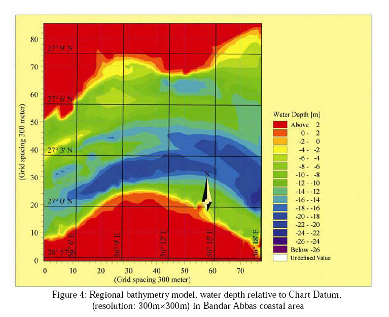
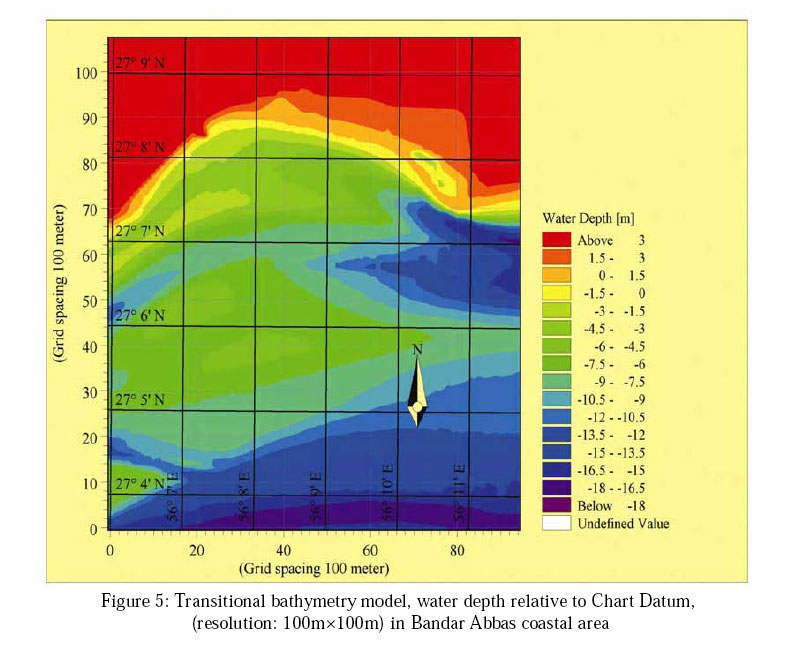
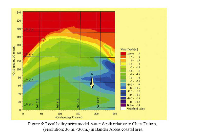
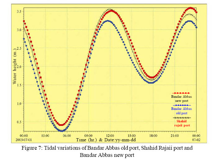
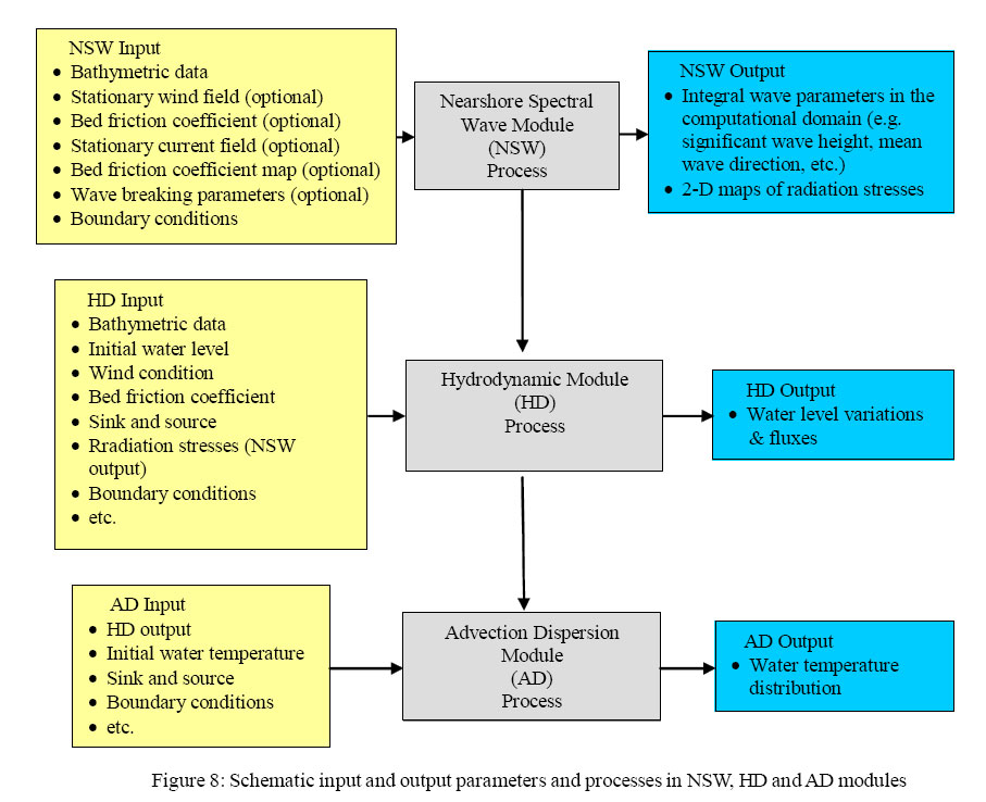
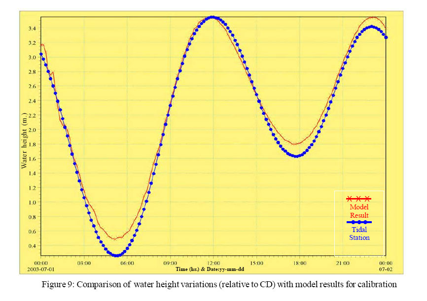
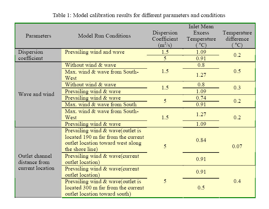
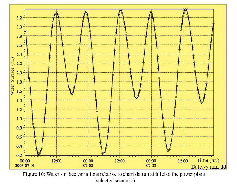
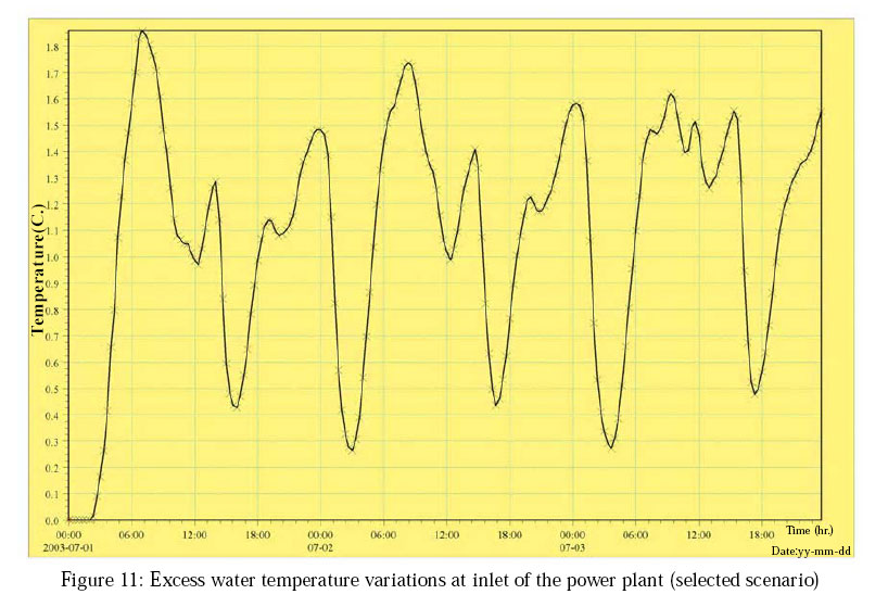
Selecting model area and grid spacing

For hydraulic modeling, three areas about 25km×25km (regional model), 12km×14km (Transitional model), 7 km.×7 km. (local model) with grid spacing respectively 300 m.×300 m., 100 m.×100 m. and 30 m. ×30 m. are chosen in order to transfer the water velocity and height from each larger model to the open boundary of the smaller one (Figures 4, 5 and 6). For wave modeling, the grid spacing for transitional model is 100 m.×300 m. and for local one is 30 m. ×30 m. The largest model is extended such that there is a tidal station nearly at each end of the open boundaries. The transitional model is extended in which the flow pattern due to wave and wind to be computed, and the local model is extended to encompass the heated area thoroughly.

Boundary conditions

As mentioned previously, there are tidal stations at the open boundaries of regional model. So, the water surface elevation data from tidal stations is specified at the open boundaries to execute the hydrodynamic model run. At transitional model open boundaries the required boundary conditions (water level variations and fluxes) are transferred from regional hydrodynamic model output.

Besides, in this area, wave parameters are specified at the offshore boundary of the region in NSW module. After executing the local NSW model run, the wave parameters are extracted as input for NSW local model in order to compute the radiation stresses (as input for local hydrodynamic model).

At local model open boundaries the required boundary conditions are transferred from transitional model to open boundaries. Hydrodynamic and heat transfer modeling in the local area is carried out at the same time. In this area at the open boundaries, as the temperature data is not sufficient, the mean water temperature is specified.

Model calibration/verification

In order to rely on the results of any modeling study, the model should be calibrated and verified to a satisfactory accuracy. In the following the calibration and verification of the models are described:

1. Hydrodynamic model calibration/verification

Tidal variation data for three stations was available. Two stations locate nearly on the open boundaries of the largest model.In the following the calibration and verification of the models are described:

The data was applied for one day on the open boundaries and after simulation; the extracted data from model at the third station was compared with the real data.

The model was calibrated by changing the bed resistance factor until the error is less than 15 percent regarding the real data mean value. For verification, the data was applied for two other days on the open boundaries without changing any factor; after simulation, the error was less than 15 percent and it wasn’t necessary to carry out any verification. The result for calibration is shown in Figure 9.

2. Advection Dispersion model calibration / verification

Considering that the excess temperature in the inlet channel is not to be more than a specific value (in order to prevent decrease in power plant efficiency), the simulation was carried out with different scenarios, mentioned bellow, in which the highest tidal variations in the year occur (in order to discover the worst condition in inlet due to hot water recirculation).

• Model run, considering the tidal variations, without considering the wind and wave.
• Model run, considering the tidal variations and maximum southwest wind and wave.
• Model run, considering the tidal variations and prevailing south wind and wave; by considering different locations for discharging the hot water at the current outlet location, in the sea and along the shoreline.
• Model run, considering the tidal variations and max south wind and wave. There were not enough water temperature data to calibrate the model and to determine the heat dispersion coefficient. Therefore, in order to find out how much the dispersion coefficient affects the inlet temperature, the simulation was carried out by different dispersion coefficient values.According to these simulations, it was concluded that various dispersion coefficients have little effect on inlet temperature, and it does not affect on the simulation results so much (Table 1).

3. Wave model calibration/verification

As no wave measurements were available, no calibration was carried out. However, temperature variations due to various wind and wave conditions show a little effect on the inlet temperature (Table 1).

Results

Model results

• The max south-west wind and wave (causing the critical situation in inlet) makes an increase 2.5 ^oC at the inlet water temperature, at maximum. Increasing the outlet distance from inlet and moving toward the sea or along the shoreline, can cause a decrease in inlet water temperature (Table 1).
• At the end of the low water (ebb) and beginning of high water (flow) the highest temperature occurs at the inlet (Figures 10 and 11).
• Although the highest temperature occurs in simulation with considering the tidal flow and max south-west and west wind and wave, these scenarios were not used to determine the outlet distance from inlet (because of the little frequency of their occurrence –about 1 percent), and the best scenario for outlet distance determination is on the basis of simulation with considering the tidal flow and prevailing wind and wave (see Figure 12 for its excess water temperature distribution at Bandar Abbas power plant coastal area).
• Temperature variations in inlet, due to dispersion coefficient variations is little (about 0.2 -0.5 ^oC). Consequently, determination of distance between outlet and inlet is on the basis of the scenario in which tidal flow with prevailing south wind and wave is considered. This scenario shows higher water temperature (as mentioned below) than the real situation. Therefore, the results obtained from it define the worst condition at the inlet; and the outlet channel distance to the inlet can be determined.

1. In the hydrodynamic simulation the time series tidal flow data and a constant value for wind and wave is used. The constant value magnifies the effect of the wind and wave, and increases the max inlet water temperature more than real situation.
2. The model is 2D and heat dissipation is not due to mixing with the lower layers of the water, and heat dissipation is only to the atmosphere. Therefore, the simulation show higher values comparing the real situation.
3. The simulation was carried out for one day with highest water variations (ebb and flow), So, It magnifies the inlet water temperature more than the real situation.

Economical comparison of different alternatives for discharging cooling water into the sea in BATP development plan

The most important part in each project is to choose a cost-effective alternative. In this survey, to discharge the cooling water, three following alternatives are compared as of economical aspects.

• Construction of an outlet channel which is 500 m. in length in BATP development plan parallel to the current outlet, which costs 634147, 8 USD.
• Construction of three parallel outlets for discharging the whole water -used by the power plant - which is 690 m. in length (the discharge location is 190 m. far from the current outlet along the shoreline toward west), which costs 1384797, 8 USD.
• Construction of an outlet which is 500 m. in length for discharging the excess discharge (in BATP development plan) and parallel to the current one; and pipe laying is 300 m. in length in to the sea toward south to discharge the whole amount of cooling water, which costs 5118548 USD (pipe laying under the sea has the most effect on cost growth).

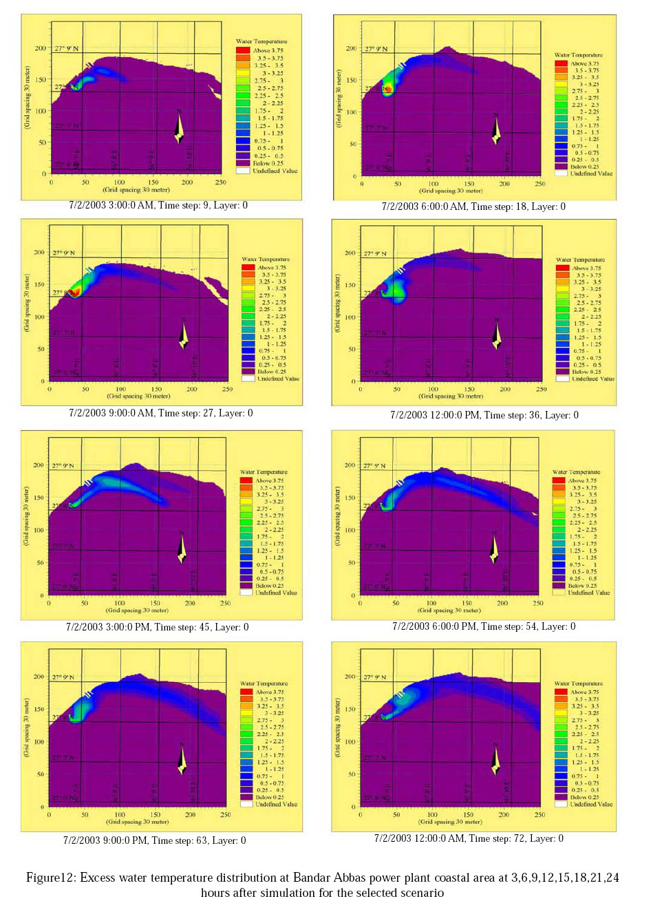
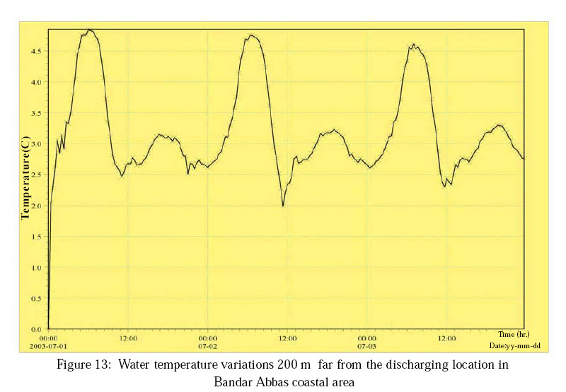
As it was expected, the first alternative is the cheapest and most effective one.

Discussion and Conclusion

After reviewing simulation results, the scenario considering the prevailing south wind and wave without changing the current location of the outlet causes the greatest excess temperature in the inlet, and either the temperature does not exceed more than an allowed amount. In addition, construction of an outlet channel (500 m. in length) parallel to the previous one, and construction of a structure for discharging the added flow (in BATP development plan) into the sea is the cheapest and the most costeffective one. Therefore, the location of the outlet adjacent to the current one is recommended for discharging cooling water in this project.

Thermal pollution environmental assessment in BATP development plan

According to theIranian Department of the Environment (DOE) standardsthe hot water discharge into a water resource must not make an increase in the water ambient temperature more than 3 degrees Celsius in a distance equal to 200 m. far from the discharging location. The model result shows that the water temperature in Bandar Abbas coastal area exceeds than the permissible limit and in order to decrease its harmful impacts, some considerations, mentioned below, should be applied (Figure 13).

In order to simulate each phenomenon by software, it is necessary to collect various data for a long period of time to use them as an input for the model. In this research, lack of data was the basic problem.

Availability of a complete time series data is too important to accomplish a simulation properly and to use the results of these basic models for later predictions and purposes. The final goal of data collection is to calibrate and verify a simulation. Therefore, the data -mentioned below-is necessary to be collected for Bandar Abbas region from meteorological stations in land and sea, and buoys: Wind direction and velocity, precipitation, evaporation, water temperature, water flow direction and velocity, wave conditions such as height, period, and direction and so on.

There are various methods to reduce and control the thermal pollution problem. Among which are: using the cooling towers -not recommended in this project because of existence of high amount of dissolved matters in the sea water that can be deposit in the pipes-, dilution through the outlet way by adding sea water that it does help to reduce the temperature, discharging the cooling water into the ponds for some time to get cooler, and finally, dividing the cooling water amount and discharging each portion of it in different locations to reduce its harmful effects.

Acknowledgments

Special thanks to Danish Hydraulic Institute (DHI) for providing MIKE 21 model.

References

• Ekebjaerg, L. and P. Justesen, An explicit method scheme for advection-diffusion modeling in two dimensions. Computer methods in applied mechanics and engineering, North Netherlands, 88: 287-297, 1991
• Kummar, U. and B. Kakrani, Water, Environment and Pollution, Agrobios, India, 2000
• Mahboob-ul-Kabir, M., Past Studies and Further Scopes on Wave modeling in the Coastal Region of Bangladesh, Conference proceedings of the 1^st Asia Pacific DHI Conference, Bangkok, 2002
• MIKE 21 Environmental Hydraulics Advection, Dispersion Module, scientific Documentation, DHI Software, 2003
• MIKE 21 Environmental Hydraulics Advection, Dispersion Module, Reference Manual, DHI Software, 2003
• M. Abbaspour, et al.
• MIKE 21 Coastal Hydraulics and Oceanography, Hydrodynamic Module, Scientific Documentation, DHI Software, 2003
• MIKE 21 Nearshore Spectral Wind-Wave Module, Scientific Documentation. DHI Software 2003
• Samadi, R., Correlation assessment of management and planning with the environment in Bandar Abbas power plant, Master of science thesis, Tehran University, 1997
• U.S. Army corps of Engineers, Engineering and Design Coastal Inlet hydraulics and Sedimentation, Manual No.1110-2-1618, 1995
• Zahid, M. A. and Z. Mohammadi Dashtaki, Marine Pollution, Nagshe MehrPublication, 2000

© 2005 Center for Environment and Energy Research and Studies (CEERS)

The following images related to this document are available:

Photo images