 |
| About Bioline | All Journals | Testimonials | Membership | News |
|
||||||
|
||||||
International Journal of Enviornmental Science and Technology, Vol. 2, No. 3, Autumn, 2005, pp. 259-267 Daily air pollution time series analysis of Isfahan City 1R. Modarres and 2*A. Khosravi Dehkordi 1Faculty of Natural Resources, Isfahan University of Technology, Isfahan, Iran 2Department of Environmental Sciences, Graduate College of Natural Resources, Isfahan University of Technology, Isfahan, Iran Received 25 May 2005; revised 11 June 2005; accepted 18 July 2005; onlined 30 September 2005 Code Number: st05036 Abstract Different time series analysis of daily air pollution of Isfahan city were performed in this study. Descriptive analysis showed different long-term variation of daily air pollution. High persistence in daily air pollution time series were identified using autocorrelation function except for SO2 which seemed to be short memory. Standardized air pollution index (SAPI) time series were also calculated to compare fluctuation of different time series with different levels. SAPI time series indicated that NO and NO2, CH4 and non-CH4 have similar time fluctuations. The effects of weather condition and vehicle accumulation in Isfahan city in cold and warm seasons are also distinguished in SAPI plots. Key words: Air pollution, time series, ACF, non linear dynamic, SAPI, Isfahan Introduction The limitless of air pollution range and sources have forced pollution managers to apply new methods in air pollution control and monitoring. Development and use of statistical and other quantitative methods in the environmental sciences have been a major communication between environmental scientists and statisticians (Herzberg and Frew, 2003). This approach is called top-down approach which starts with statistical analysis of collected air pollution data (Lee, 2002). In recent years many statistical analysis have been used to study air pollution as a common problem in urban areas. The common descriptive statistical approach used for air quality measurement and modeling is rather limited as a method to understand the behavior and variability of air quality. Different techniques have been used for air quality monitoring systems. Voigt et al., 2004 applied principle component analysis in order to evaluate different air pollutants like ozone (O3), nitrogen dioxide (NO2) and carbon monoxide (CO) in 15 European member states. Many investigators have used probability models to explain temporal distribution of air pollutants (Bencala and Seinfeld, 1979, Yee and Chen, 1997). Time series analysis is a useful tool for better understanding of cause and effect relationship in environmental pollution (Schwartz and Marcus, 1990, Salcedo et al., 1999, Kyriakidis and Journel, 2001). The principle aim of time series analysis is to describe the history of movement of a particular variable in time. Many authors have tried to detect changing behavior of air pollution through time using different techniques (Salcedo et al., 1999, Hies et al., 2000, Kocak et al., 2000, among others). Many others have tried to relate air pollution to human health through time series analysis (Gouveia and Fletcher, 2000, Roberts, 2003, Touloumi et al., 2004). The object of this study is to examine daily time series analysis of some air pollutants in Isfahan City, in the center of Iran. The average daily air pollution concentrations (APC) of SO2, CO, CH4, NO2, NO, non-CH4 and O3 were selected from March 2003 to March 2004. Material and MethodsDescriptive analysis The classical descriptive analysis is the first statistical analysis dealing with any data. Mean, standard deviation (STDEV), maximum and minimum value of selected data sets are usually calculated to have preliminary knowledge of selected variables. The calculation of coefficient of variation (cv) helps the investigator to overcome the problem of different levels and units of variables in order to compare them. Coefficient of Skewness (cs) and Kurtosis (ck) are other measures which may be used to characterize the symmetry and flatness of the probability density function of a time series, respectively (Windsor and Toumi, 2001). Because of high order, kurtosis is particularly sensitive to extremes or intermittent fluctuations and, therefore, a useful indicator of intermittency. Highly intermittent time series have a higher kurtosis. However, descriptive analysis is of rather limited value due to the large variability associated with air quality data through time (Salcedo, et al., 1999). Time series analysis A time series is a set of observations that are arranged chronologically. In time series analysis, the order of occurrence of the observation is crucial. If the chronological ordering of data were ignored, much of the information contained in time series would be lost. A variety of different important terminologies in time series analysis are existence such as stationarity, periodicities and trend which fall into temporal categories of air pollutant concentration (Klemm and Lange, 1999, Lee, et al., 2003). Stationarity of a process can be qualitatively interpreted as a form of statistical equilibrium. Therefore, the statistical properties of the process are not a function of time. For interpretation purposes, it is often useful to plot Autocorrelation function (ACF) against lag time, K. ACF is a simple graphical method to find time relationship of an event. The sample autocorrelation coefficient is written as (Box and Jenkins,1976):
Where N is the total length of record, K is lag time,Xt is observation at time t and
Where β0 to βp are the parameters of regression equation and least square point estimates of them may be obtained by using regression techniques. For statistical inference on the significant of regression and parameters, the reader is referred to Bowerman and O’connel (1993). Standardized time series The above analysis will show us whether air pollutant are dependent on time or not but in air pollution time series analysis, it would be useful to find time periods of risky air pollution levels. In order to compare different air pollutants with different levels and units, we use standardized air pollution index which is written as follows:
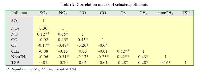
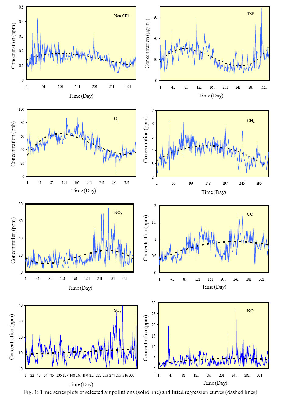
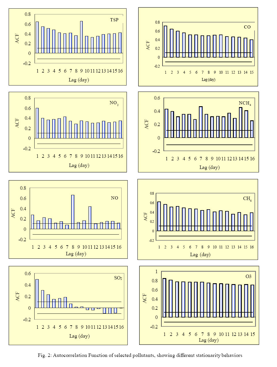
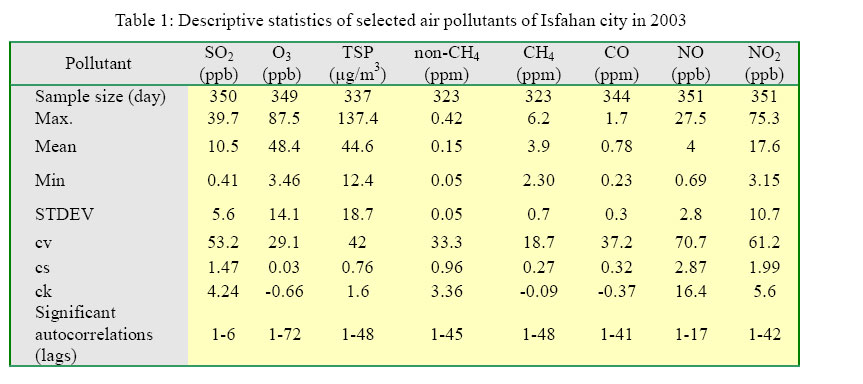
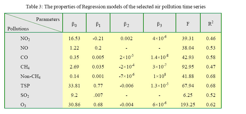
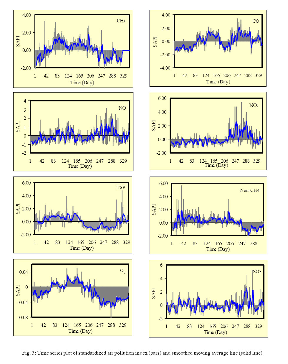
WherePi is the pollutant concentration at time i, P and σ are the mean and standard deviation of the series and SAPI is the StandardizedAir Pollution Index. Standardized air pollution index is not only useful to determine risky periods of air quality characteristics but to define the risky periods as well. It is also possible to determine air pollution interaction through time using cumulative SAPI. The ASAPI will disclose the cumulative risky periods of air quality and is useful in air health monitoring. Results Descriptive analysis The descriptive statistics of selected daily air pollutions are presented in Table 1. As the coefficient of variation (cv) is a measure of variation over time (Lee, 2002), the comparison of pollutants indicates that NO has the highest variation over time while CH4 has the smallest variation. The degree of variation decrease in the order: NO< NO2< SO2< TSP < CO < non-CH4 < O3 < CH4. This variation may be the result of variation in generating resources or weather condition. The coefficient of skewness (cs) measures the relativse skewness of frequency distribution; as time series, air pollution concentration data are characterized buy strongly right-skewed frequency distribution in this study like other previous studies by Georgopoulos and Seinfeld (1982) and Lee (2002). The degree of rightskewness decrease in order: NO < NO2 < SO2 < non-CH4 < TSP < CO < CH4 < O3. The higher ck of most of the pollutants indicates intermittency in most of air pollutants, except for CH4, CO and O3. Non-CH4 is perhaps the nearest air pollutants to Normal distribution with cs=1 and ck=3. The degree of kurtosis decrease in order: NO < NO2 < SO2 < non-CH4 < TSP < CH4 < CO < O3. Perhaps the most interesting result of descriptive analysis is small value of cs and ck of O3. It is well known that high O3 concentration is produced only when sunlight is strong (almost during summer in Isfahan city). Therefore it is assumed that the difference between low and high concentration is large, resulting in the largest skewness and variation in all examined air pollutants (Lee, 2002). The result of this study is exactly in the opposite, where O3 has the minimum values of skewness and variation. The correlation matrix (Table 2) also indicates the time correlation between different pollutants. High, positive correlations between chemically-similar pollutants like NO2 and NO, CH4 and non-CH4 are appealing. The positive correlation indicates synchronous time fluctuations of air pollutants. The different time correlation behavior of the pollutants is further discussed in section 3.3. Time series results The first step in time series analysis is to draw time series plot. Time series plot can give a preliminary understating of the time behavior of the series. Fig.1. shows time series plot of selected time series air pollution concentration. This Figure shows different time behavior of air pollutants. For example, the concentration of O3 and TSP seem to have a similar trend from the beginning of the year to the end but the maximum and minimum concentrations occur in different time. It is also obvious that SO2 and NO have not a significant trend through time. The fluctuations of NO2, SO2 are more irregular at the end of the year but the fluctuation of non-CH4 is more obvious at the beginning of the year. The autocorrelation functions of the selected time series also show different time stationarity of the series. The autocorrelation functions of them are presented in Fig. 2. The significant lags for all selected pollutants are also presented in Table 1. Except for SO2, all other pollutants show nonstationarity (long serial correlation). The amplitude of autocorrelation functions do not become less pronounced for most of the series, except for SO2. This is an indication that the memory of SO2 is finite. Time series regression was applied to the selected series. The significant time regression was selected based on R-Square and F-statistics. Statistical inference for regression parameters was done based on null hypothesisH0 : β1 =β2 =... =β0 =0 and all parameters were significant at α= 95%. The parameters of regression models are presented in Table 3 while they are graphically presented in Fig. 1. Except for SO2 and NO, it is clear that most of the air pollutions follow a non linear trend through time. The non linear time dynamic of air pollution is probably the result of non linear behavior of pollution generating mechanism or weather fluctuations. This non linearity behavior was also identified by other investigators such as Kocak et al., 2000, Salcedo et al., 1999 and Hies et al., 2000. The linearity of NO and SO2 also matches stationary condition of the series indicated in Table 1. In other words, the mean concentration of SO2 and NO does not vary through time. SAPI time series For analyzing air quality data, it is very important to find the periods with adverse effect on public health (Gouvvia and Fletcher, 2000, McKee et al., 1993), even at historically low level of air pollution (Touloumi et al., 2004). In order to find these periods, standardized air pollution index was calculated and presented in Fig. 3. The figure shows that the fluctuation of air pollution differs through time. For example, NO2 does not differ from zero for 219 (spring and summer) days but the concentration is significant after that. In other words, the adverse level of NO2 appears mostly at the end of the year. This may occur due to increase in gasfired home heating systems in winter. In contrast, O3 has negative values of SAPI at the end of the year, approximately after day 219. This is the result of inverse correlation between NO2 and O3 (Table 2) which indicates the interaction of O3 as a secondary pollutants and NO2 as the primary pollutants. Because O3 is an oxidizing chemical and its production requires the presence of sunlight, high levels of O3 occurs in summer (Fig. 1). SO2 is again attractive air pollution as the fluctuation of SO2 around zero is approximately symmetric and intermittent. SO2 highest values of SAPI’s are observed between 270 to 290 days. The main source of SO2 emission in Isfahan city is intermittent road transport of diesel vehicles and large power stations and industrial process around the city. Other air pollutants indicate different periods of high and low SAPI. The comparison of different SAPI shows the inverse time behavior characteristics of NO2 and non-CH4. Whole NO2 has negative value of SAPI at the beginning of the year to almost 220th. day, the negative values of Non-CH4 begins approximately from 240th. day. The time behavior of two hydrocarbon pollutants, CH4 and non-CH4, seems to be mostly similar to each other, except for the beginning of the year when CH4 begins to increase earlier than non-CH4. The increasing of hydrocarbon and carbon monoxide air pollutants in summer is mostly due to high vehicle concentration in Isfahan city as one of the main tourist-attracting city of Iran. Another important hydrocarbon resource is petrochemical industry in the north west of the city. The role of hydrocarbons in O3 formation can be seen in Table 2 and Fig. 3. The higher values of CO in winter are also the result of increase in home heating systems with fossil fuels. The other two related pollutants, NO and NO2 also show the same behavior. Although NO2 has negative values (low risky values) for the 220 day of the year but NO has some positive (high risky values) values between 90th. and 165th. days and then between 220th. and 300th. days. The effect of wind blowing in fall and winter is the main reason of TSP decreasing in cold seasons of Isfahan. Discussion and Conclusion Daily air pollution time series analysis of Isfahan city was performed in this study and showed different temporal behavior of different air pollutants. While some pollutants like NO2 and SO2 show simple temporal fluctuation through the year, other pollutants show high fluctuation and have mostly non linear trend through the year using time series regression. High coefficient of variation and kurtosis in most of the observed series also indicated non linearity variation of air pollutants concentration through time. Standardized time series analysis which let us compare different pollutants with different levels and units, indicates different health adverse periods from the beginning of the year to the end. This different time behavior is not only the reason of correlation of different pollutants with each other but the seasonal variation on increasing or decreasing air pollutants as well. It was also shown that most daily air pollution time series have high persistence of air pollution conditions through time. This persistence is not only dangerous for public health but also makes air pollution management and control very difficult, except for NO2 and SO2. The influence of weather conditions like rainfall, air moisture and wind velocity-direction on air pollution temporal dynamics is also very important in air pollution management and control which will be ongoing author’s task to investigate. References
© 2005 Center for Environment and Energy Research and Studies (CEERS) The following images related to this document are available:Photo images[st05036t2.jpg] [st05036t1.jpg] [st05036f3.jpg] [st05036f1.jpg] [st05036t3.jpg] [st05036f2.jpg] |
| |||||||||

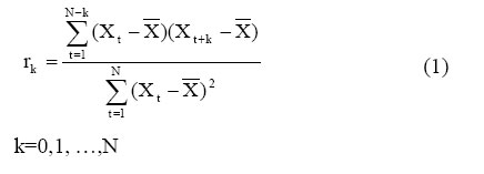
 is the mean of series. Allrk lie between -1 and +1 and values significantly above zero denote correlation at the given lag. ACF can also tell us whether the observation depends on time or not. When ACF decays rapidly to zero after a few lags, it may be an indication of stationarity in the series, while a slow decay of ACF may be the indication of nonstationarity (Salas, 1993, Hipel and McLeod, 1994). Strict stationarity means that there is no systematic change in mean (no trend), no systematic change in variance, and strictly periodic variations have been removed. Quantitatively, this means that the joint distribution of X(t1), …, X(tn) is the same as the joint distribution of X(t1+t),….,X(tn+t), for all t1,…tn. This means that shifting the time origin by t has no effect on the joint distributions, which only depend on the time intervals between t1,t2,…,tn. Second-order stationarity for weak stationarity. In other words, a finite memory of the series leads to a gradual decline of the envelope of the ACF (Klemm and Lange, 1999). Another way to investigate whether a series is time dependent or not is time series regression (Bowerman and O’Connell, 1993). The polynomial time regression between dependent variable, yt and time is written as follows:
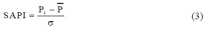