International Journal of Environment Science and Technology Center for Environment and Energy Research and Studies (CEERS) ISSN: 1735-1472 EISSN: 1735-2630 Vol. 3, Num. 3, 2006, pp. 243-250

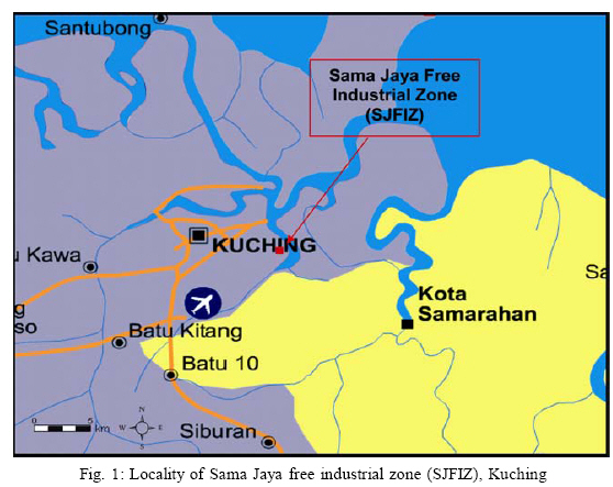
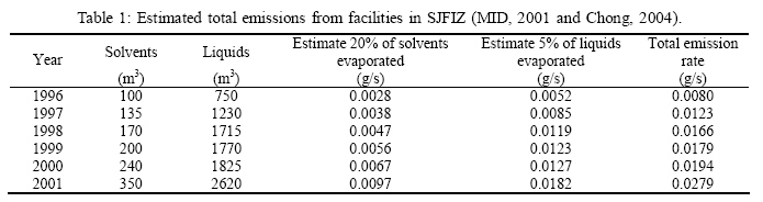
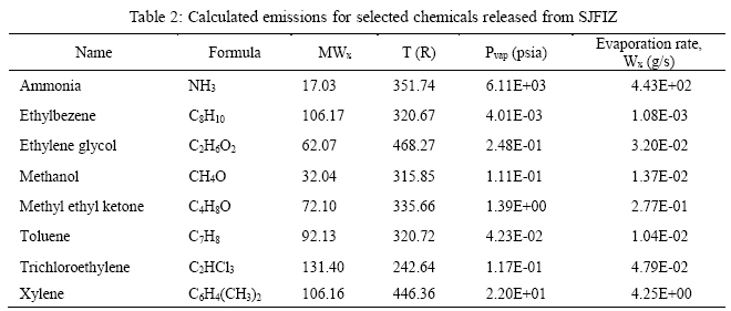
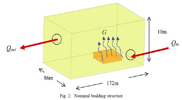
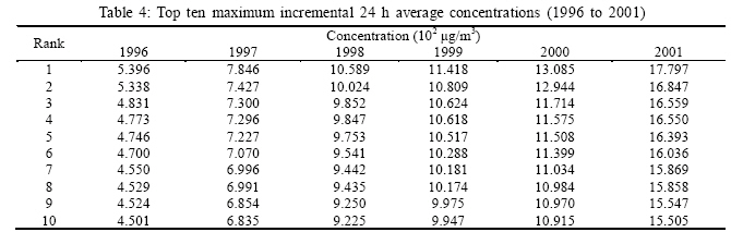
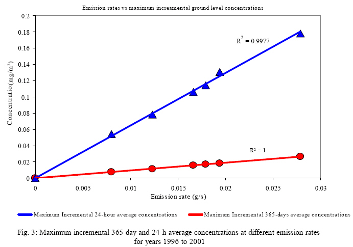
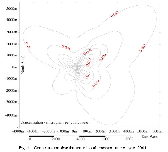
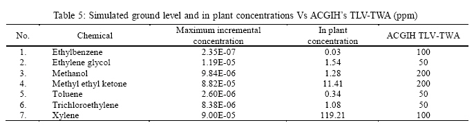
International Journal of Enviornmental Science and Technology, Vol. 3, No. 3, Summer 2006, pp. 243-250

A comparison of nearby incremental ground level and in plant concentrations of air pollutants emitted from electronics facilities

^*P. L. Law, S. C. Gracie Chong, A. Baharun and A. Abdul Rahman

Department of Engineering, University of Malaysia Sarawak (UNIMAS), Kota Samarahan, Sarawak, Malaysia

*Corresponding author, Email: puonglaw@feng.unimas.my Tel.: +6082-672 317; Fax: +6082-672 317

Received 22 March 2006; revised 25 May 2006; accepted 5 June 2006; available online 25 June 2006

Code Number: st06031

ABSTRACT: Air dispersion modeling by was recently conducted to predict the incremental ground level and inplant concentrations of toxic organic chemicals due to stack and fugitive emissions from Sama Jaya Free Industrial Zone (SJFIZ), Kuching, Sarawak, Malaysia. Simulations of organic air pollutants emitted from industrial facilities in SJFIZ from years 1996 to 2001 were carried out in September 2004 by members of Faculty of Engineering, Universiti Malaysia Sarawak (UNIMAS). The results indicated that there were negligible amount of maximum incremental ground level concentrations of less than 3x10^-2 µg/m³ for 365-day average, and less than 18x10^-2 µg/m³ for 24 h. average. For in-plant maximum incremental concentrations, it is found that the simulated results were much lower than TWA values, except xylene. The predicted in plant concentration of xylene was 119.21 (parts per million) ppm as compared to ACGIH TLV-TWA of 100 ppm approximately 19% higher than ACGIH recommended values. From this study, it was concluded that both nearby population and in plant workers were not potentially at risk to exposing organic chemicals far lower than the threshold limit levels set by ACGIH.

Key words: Incremental, ground level, in plant, air pollutants, emission

INTRODUCTION

The Sama Jaya Free Industrial Zone (SJFIZ) is located at Muara Tabuan, Kuching, Sarawak, Malaysia (01^o28’33.3"N, 110^o19’28.2"E) which will be developed exclusively by electronics, electrical and other related industries (MID, 1996 and 2001). The area of this industrial zone, which is by Sungai Kuap, is approximately 330.5 hectares (MID, 1996 and 2001). As shown in Fig. 1, theSJFIZ is approximately 6 km away from the centre of Majlis Bandaraya Kuching Selatan (MBKS) or City of Kuching (MID, 1996). Nine approved industrial facilities have been established in SJFIZ until now. The nearest residential area at Muara Tabuan is less than one kilometre away from the industrial zone and the health risk impacts are expected to be present due to the magnitude of the production (MID, 1996). However, the air pollutants emitted from the industrial facilities could be hazardous to the nearby population and in plant workers (Gracie Chong, 2004). Most of the industrial wastes generated from SJFIZ are in solid, semi-solid and liquid forms, e.g., solvent, oil, sludge, liquid and solids wastes (Gracie Chong, 2004). However, most of the solvents and liquids are volatile, like the organic degreasing solvent (methylene chloride, perchloroethylene, trichloroethylene, 1, 1, 1trichloroethane and trichlorotri-fluoroethane) (MID, 2001 and Gracie Chong, 2004). Based on the data supplied by electronics facility operators located in SJFIZ, it was estimated that about 20% of the volatile solvents and 5% of liquids were evaporated and emitted into the atmosphere during operation as indicated by the differences between the amount solvents/liquids purchased and disposed off as liquid wastes (Gracie Chong, 2004). Based on the program and developed area, the assumed quantity of chemical used in process line from the SJFIZ is shown in Table 1 (MID, 2001). The monthly waste total emissions from the industrial facilities in SJFIZ are shown in Table 1, and the primary organic degreasing solvents air emissions from SJFIZ are ammonia, ethylbenzene, ethylene glycol, methanol, methyl ethyl ketone, toluene, trichloroethylene and xylene (Gracie Chong, 2004). The estimated total air emissions SJFIZ industries are presented in Table 1, and estimated emission rates by engineering calculation methods for major chemicals are shown in Table 2 (Gracie Chong, 2004). However, most of the solvents and liquids are volatile, such as the organic degreasing solvents such as methyl ethyl ketone, toluene, xylene and methanol (MID, 1996). The estimated total emissions released into the atmosphere from SJFIZ industries are given in Table 2. To estimate the selected chemicals encountered in semiconductor manufacturing industries in SJFIZ, the estimated emission rates using engineering calculation methods for selected chemicals are shown in Table 2 (MID, 2001 and Gracie Chong, 2004).

MATERIALS AND METHODS

In this study, computer simulations using Industrial Source Complex Short Term (ISCST) developed by United States Environmental Protection Agency (US EPA) was carried out in an attempt to determine nearby ground level incremental organic chemical concentrations released from SJFIZ through stack and fugitive emissions within a radius of 6 km from emission source (US EPA, 1986 and 1993). In plant air pollutant concentrations were modeled based on the typical structure of the facilities, amount of in plant fugitive emission rates, volume of buildings, and the type of exhaust ventilation systems. Incremental air pollutants at ground level were then compared against the in plant pollutant levels.

Atmospheric air dispersion modeling

The ISCST was developed by USEPA and is a regulatory model for both the State and Federal governments of the United States of America (Zoch and Egan, 1988). The ISCST air dispersion model is a steady-state plume model, which can be used to assess pollutant concentrations from wide variety of sources, associated with industrial source complexes. This model also accounts for settling and dry deposition of particulate, downwash, area, line and volume sources, plume rise as a function of downwind distance, separation of point sources, and limited terrain adjustment (US EPA, 1995). The ISCST is designed to calculate the average seasonal and/or annual ground level concentration or total deposition from multiple continuous point, volume and/or areas sources. Provision is made for special discrete, X, Y receptor points that may correspond to sampler sites, points of maximum or special points of interest. Some of the major factors considered in analysing air quality impacts of emissions from industrial source complexes are stack emissions, hourly meteorological information, and timedependent exponential decay of pollutants, dry deposition, and gravitational settling (US EPA, 1995). The meteorological conditions over the industrial facilities include the mean surface air temperature; mean and maximum surface wind speed and direction obtainable from Malaysian Meteorological Service (MMS). The ISCST air dispersion model was chosen as one of the key components of this model that uses the meteorological information on a h-by-h basis. The ISCST is deemed a suitable for assessing pollutant concentrations from the wide variety of sources associated with industrial complexes (US EPA 1986 and 1993). The hourly weather data contains wind speed, wind direction, temperature, atmospheric stability, and mixing heights (US EPA, 1995). PCRAMMET is a preprocessor program that provides and merges all the datasuch as hourly stabilityclass, wind direction, wind speed, ambient temperature and mixing height for use in ISCST (US EPA, 1995). It processes input data formats including hourly surface observations, twice-daily mixing height data, and precipitation data. The data input files for running PCRAMMET are mixing height data and hourly surface meteorological data. For pollutant concentration estimation, the necessary mixing height data required are National Weather Service (NWS) Station Number, year, month, day, morning mixing height values and afternoon mixing height values (US EPA, 1995). All those data are arranged in a specified column in a file with extension .mix. The variables used by PCRAMMET are NWS station, year, month, day of record, h, ceiling height, wind direction, wind speed, drybulbtemperature, total cloud cover and opaque cloud cover. Those data are properly arranged in a file with extension .srf (US EPA, 1995). The data offered in the mixing height data files comprise of data provided by the Malaysian Meteorological Service in their “Twice Daily Mixing Height Data” format. The format of the records has been modified to correspond to that required by the PCRAMMET pre processor programs. In addition, the first and last records of each file have been added to conform to the requirements of these pre-processor programs. PCRAMMET also requires that the meteorological input data sets contain no missing values (US EPA, 1995).The processing ofhourly mixing heights requires morning and afternoon estimates of mixing heights, the local standard time of sunrise and sunset and hourly estimates of stability. Two interpolation schemes are used to estimate hourly mixing heights, one for rural sites and the other for urban sites. Both estimates are included in the PCRAMMET output file. The time of sunrise and sunset are calculated within PCRAMMET based on the date, latitude, longitude, and time zone, using known earthsun relationships (US EPA, 1995). In this study, the ISCST model simulated incremental ground level pollutant concentrations for 365 days average and 24 h average by using 2000 meteorological data over SJFIZ. The incremental ground level pollutant concentrations (C_i) for 365-dayaverageconcentrations and 24 h. average concentrations were simulated based on meteorological data for year 2000. To meaningfully estimate the nearby population exposure, the isoconcentration curves (isopleths) of the individual air pollutants are taken within a radius of 8 km are plotted corresponding to lowest concentration cut-off point of 0.002 µg/m³ (Law, 1993).

Estimation of in plant concentration (C_f)

One of the primary factors in determining the rate of contaminant build-up or respective contaminant levels in a facility is the type of exhaust ventilation installed (US EPA, 1988). To facilitate calculations of contaminant levels in the facility due to vapor pressures or volatilities of chemical compounds, the targeted facility buildings are assumed to be equipped with general exhaust ventilation systems. A single model of the facilities is illustrated in Fig. 2. The box represents the typical physical structure of the facilities under study, with the fugitive emission rate (G) in grams/second (g/s), volume of the building (V) in cubic meters (m³), and theair is exhausted at a volumetric rate (Q) in cubic meters per second (m³/s). For predicting general exhaust ventilation performance, which in terms would determinethecontaminant levelswithin the facility, several assumptions made include, a) pollutants are removed from the facility solely via general exhaust ventilation; b) there is perfect mixing of pollutants and air in the facility, and thus, the factor for complete mixing (K) is equal to one; and c) the exhaust ventilation rate is 10 air changes per h (US EPA, 1988).This is aimed at determining annual average concentrations to which workers are potentially exposed to the individual chemical compounds emitted within a facility as fugitive emissions. With known ventilation rate (Q) and contaminant generation rate (g/s), a constant concentration (mg/m³) could be derived by starting with a basic material balance equation as illustrated in Fig. 2. The rate of accumulation is the net value of the rate of generation minus the rate of removal as follows:

where V = volume of building (m³); G = generate rate (g/s); Q_in = amount of replacement air (m³/s); Q_out = amount of exhaust air (m³/s); C_f = concentration of pollutant, gas or vapour (g/m³); and t = time (s). To account for incomplete mixing within the facility, a K value ranging from 1 (perfect mixing) to 10 (poor mixing) is introduced to modify the rate of ventilation, and

Q’ = Q/K = effective ventilation rate (m³/s); and K = a factor to allow for incomplete mixing. In this model, a default size of a nominal manufacturing facility is (172 m x 86 m x 10 m) = 147 920 m³, and the air change rate per h (ACPH) was calculated to be approximately 10. Thus, the actual ventilation rate, Q is [147,920/ (10×60min×60s)] = 4.1089 m³/s, and K value of 1 (perfect mixing assumed) and Q value of 4.1089 m³/s were used. Concentrations of pollutants can be expressed in units of mass per unit volume (µg/m³) or in terms of a volumetric ratio (ppm, volume of contaminant per million volumes of air).

RESULTS

The ISCST model simulated the incremental ground level pollutant concentrations (μg/m³) downwind and within 8 km radius from the source area (SJFIZ) for 365- day average concentrations and 24 h average concentrations. Table 3 shows the top ten maximum ground level incremental annual average concentrations in the vicinity of emission source for years 1996, 1997, 1998, 1999, 2000 and 2001. In year 1996, the maximum annual average concentration was 0.758x10² μg/m³ occurred at 212.13m east and 212.13m north of the pollutant release source. The simulated second maximum average concentration was 0.677x10² μg/m³ occurred at 353.55m East and 353.55m north of the emission source. The maximum incremental ground level annual average concentrations were 1.157x10²μg/m³ for 1997, 1.562x10²μg/m³ for 1998, 1.684x10² μg/m³ for 1999, 1.837x10² μg/ m³ for 2000, and 2.625x10² μg/m³ for 2001. Table 4 provides the top ten maximum incremental 24 h average concentrations (μg/m³) at ground level in the vicinity of SJFIZ from year 1996 to 2001. The maximum 24 h average concentration in year 1996 was estimated to be 5.396x10²μg/m³ occurred on 72nd day at 353.55m east and 353.55m north of emission source. In years 1997, 1998, 1999, 2000 and 2001, the maximum incremental average concentrations were predicted to be 7.846 x10² μg/m³, 10.589 x10² μg/m³, 11.418 x10² μg/m³, 13.085 x10² μg/m³ and 17.797 x10²μg/m³, respectively. Fig. 3 illustrates the summary of emission rates, the maximum incremental 365 days and 24 h average ground level concentrations for year 1996 to 2001. The estimated total emission rates of the individual organic chemicals emitted from SJFIZ for year 1996 to 2001 ranged from 8 mg/s to 28 mg/s. Fig. 4 graphically illustrates the simulated incremental ground level concentration distribution of total emission rate in year 2001. Based on the simulated results, the incremental ground level concentrations increased tremendously from 1996 to 2001. The coefficients of correlation (R2) between the emission rate versus maximum incremental 365-days, and emission rate versus 24 h average ground level concentrations were found to be 1.0 and 0.9977, respectively. This indicates that the ground level concentrations are highly dependent on pollutant emission rates. In this study, a comparison was made on maximum incremental annual average ground level and in plant concentrations versus American Conference of Governmental Industrial Hygienists (ACGIH’s) Threshold Limit Values (TLV) Time Weighted Average (TWA). The maximum ground level incremental concentrations and in plant concentrations of chemicals are shown in Table 5.

The ACGIH has suggested Threshold Limit Values (TLVs) - Time-Weighted Average (TWA) permissible air concentrations of a given chemical to which an individual can be repeatedly exposed for 8 h per day, 5 days per week (Anonymous, 1988 and Sax, 1983). It is found that the simulated results are much lower than their TWA values, except the in plant concentration of xylene. The predicted in plant concentration of xylene is 119.21 ppm as compared to ACGIH TLV-TWAof 100 ppm-approximately 19% higher than ACGIH recommended values. To protect in plants workers from being exposed to excessive levels of xylene vapors, efficient ventilation system should be introduced or emission rate of xylene should be reduced so as to maintain the level below 100 ppm. Simulations of total organic air pollutants emitted from industrial facilities in SJFIZ from years 1996 to 2001 using the ISCST air dispersion model indicated negligible maximum incremental ground level concentrations of less than 3x10^-2 ìg/m³ for 365-day average, and less than 18x10^-2 μg/m³ for 24 h average.Forinplant maximum incremental concentrations, it is found that the simulated results were much lower than TWA values, except xylene. The predicted in plant concentration ofxylene is 119.21ppm as compared to ACGIH TLV-TWA of 100 ppm approximately 19% higher than ACGIH recommended values. Thus, it is concluded that both nearby population and in plant workerswerenot potentially at risk to exposing organic chemicals higher than the threshold limit levels set byACGIH.

REFERENCES

• ACGIH, (1988). Industrial Ventilation: A Manual of Recommended Practice, 20^th Ed., Cincinnati: American Conference of Governmental Industrial Hygienists, Inc.
• Gracie Chong, S. C., (2004). A model for prediction of nearby population and in plant workers exposure to air pollutants released from industrial facilities, Masters Thesis, Kota Samarahan: Department of Engineering, Universiti Malaysia Sarawak (UNIMAS).
• Law, P. L., (1993). A model for the prioritization of toxic chemicals: Relative chemical toxicities, Chemical atmospheric fate, nearby population and in-plant workers exposure as ranking factors, doctoral dissertation, lwell: Department of Work Environment, College of Engineering, University of Massachusetts, USA.
• MID, (1996). A Conceptual Study on Disposal of Hazardous Wastes from the Sama Jaya Free Industrial Zone (SJFIZ), Ministry of Industrial Development, Sarawak, Kuching: Sarawak Government.
• MID, (2001). Sama Jaya Free Industrial Zone: Your Profit Centre in Malaysia, Ministry of Industrial Development, Sawawak, Kuching: Sarawak Government.
• Sax, N. I., (1983). Dangerous properties of industrial materials, 6^th. Ed., New York: Van Nostrand Rainhold.
• USEPA, (1986). Air Quality Planning and Standards Office, Guidelines on Air Quality Models (Revised) United States Environmental Protection Agency, EPA-450/2-78-027R, Washington D.C.
• USEPA, (1993). Selection Criteria for Mathematical Models Used in Exposure Assessment: Atmospheric Dispersion Models, Environmental Protection Agency, EPA/600/8-91/ 038, Washington D.C.
• USEPA, (1995). User’s Guide for the Industrial Source Complex Dispersion Models, Volume I-User Instruction, Environmental Protection Agency, EPA-454/B-95-003a, North Carolina.
• USEPA, (1995). User’s Guide for the Industrial Source Complex Dispersion Models, Volume II-Description of Model Algorithms, Environmental Protection Agency, EPA-454/ B-95-003b, North Carolina.
• Zoch, R. M. and Egan, B. A., (1988). Air quality handbook: A guide to permitting and compliance under the clean air act and air toxics programs, 10^th. Ed., Acton: ENSR Consulting and Engineering.

© 2006 Center for Environment and Energy Research and Studies (CEERS)

The following images related to this document are available:

Photo images