International Journal of Environment Science and Technology Center for Environment and Energy Research and Studies (CEERS) ISSN: 1735-1472 EISSN: 1735-2630 Vol. 4, Num. 1, 2007, pp. 141-149

International Journal of Enviornmental Science and Technology, Vol. 4, No. 1, Winter 2007, pp. 141-149

Single hidden layer artificial neural network models versus multiple linear regression model in forecasting the time series of total ozone

Bandyopadhyay, G. & ^*Chattopadhyay, S.

Department of Information Technology of Pailan College of Management and Technology under West Bengal University of Technology, India
*Corresponding author, Email: surajit_2008@yahoo.co.in Tel./Fax: +9198 3073 6116

Received 27 September 2006;
Revised 5 November 2006;
Accepted 2 December 2006;
Available online 1 January 2007

Code Number: st07018

ABSTRACT: Present paper endeavors to develop predictive artificial neural network model for forecasting the mean monthly total ozone concentration over Arosa, Switzerland. Single hidden layer neural network models with variable number of nodes have been developed and their performances have been evaluated using the method of least squares and error estimation. Their performances have been compared with multiple linear regression model. Ultimately, single-hidden-layer model with 8 hidden nodes have been identified as the best predictive model.

Key words: Arosa, total ozone, single-hidden-layer, artificial neural network, multiple linear regression, forecast

Processes involved in the formation of ozone (O₃) are highly multifaceted in nature. Ozone is a secondary pollutant and is not usually emanated straightforwardly from stacks. Instead is formed in the atmosphere as a result of reactions between other pollutants emitted mostly by industries and automobiles. The ozone precursors are generally divided into two groups, namely oxides of nitrogen (NOX) and volatile organic components (VOC) like evaporative solvents and other hydrocarbons. In suitable ambient meteorological condition (e.g. warm, sunny/clear day) ultraviolet radiation (UV) causes the precursors to interact photochemically in a set of reactions that result in the formation of ozone.

The process of ozone formation can be expressed as:

NO₂+ UV→ NO+O
O+O₂+M→ O₃+M

Where, M is a third body molecule that remains unchanged in the reaction.

Ozone produced this way gets simultaneously destroyed as:

O₃+D→DO+O₂

Where, D implies additional reactant that destroys the ozone via oxidation.

Because of its capability to absorb the incoming radiation, the stratospheric ozone is a major source of stratospheric heating, which further heats the troposphere. Again, because of radiation of IR the tropopause gets some cooling. Thus, stratospheric ozone exerts both heating and cooling effect on the land-troposphere system. Total ozone is a measure of the number of ozone molecules between the ground and the top of the atmosphere. In a more mathematical language, total ozone is simply the integral of the ozone concentration with respect to height. A literature survey by the authors of the present contribution has shown that statistical time series analysis approach in forecasting the atmospheric and environment pollution has been proved viable by a number of researchers (e.g. Milionis and Devis, 1994; Shi and Harrison, 1997 and many others). But, in recent times, artificial neural network (ANN) has been proposed by many scientists as a better alternative to the conventional regression approach in forecasting time series pertaining to complex atmospheric and environmental phenomena. Since formation of ozone is a highly intricate phenomenon, a number of researchers have concentrated on its prediction and consequently comparative studies have been carried out to discern the performance of ANN over conventional regression approach in predicting tropospheric ozone over different cities. Prybutok, et al., (2000), Balaguer Ballester, et al.,(2002), Nunnari, et al., (1998), Viotti, et al., (2002) put ANN into practice in a number of case studies where they established supremacy of ANN over customary methodologies in ozone forecasting. Corani (2005) implemented ANN, pruned ANN, and lazy learning to predict ozone concentration over Milan. But, in all the aforesaid works, ANN models have been developed with other meteorological variables as predictors. In none of the ANN applications to ozone concentration, past values of the same data have been used as predictor. Since all other meteorological variables have their own chaotic characteristics and complexities, their inclusion to the input set would incorporate more complexity in the forecasting. Present approach viewed the prediction problem from a different point of view. Instead of tropospheric ozone, total ozone has been considered as the predictand and instead of incorporating other meteorological variables; past values of the total ozone time series have been explored in developing ANN predictive models. Performance of ANN models has been compared with conventional regression model. The research work explained in the present paper has been done in Kolkata, India, during the periodApril-June 2006.

Artificial Neural Networks, an overview

Artificial Neural networks are mathematical analogue of biological neural systems, in the sense that they are made up of an interconnected system of nodes (neurons). Furthermore, a neural network can recognize patterns in numeric data in a similar fashion to the learning process in its biological counterpart. Neural networks are highly robust with respect to underlying data distributions (non-parametric), and no assumptions are made about relationships between variables (unlike the linear or pre-specified curvilinear relationships in regression). Since it does not depend upon any assumption regarding the data and it is robust to chaotic behavior of the data, ANN has opened up new avenues to pattern recognition and forecasting related to complex natural processes. According to Maqsood, et al., (2002) ANNs are highly suitable to the cases where the underlying processes are less recognizable and are characterized by chaotic features. Though ANN can be used in a number of complex problems, the basic jobs that can be performed byANN can be precisely enlisted as

• Pattern recognition
• Pattern classification
• Prediction

Since the present paper involves prediction problem, the features ofANN are discussed here from the point of view of prediction. The earliest trainable layered neural networks with multiple adaptive elements was the Madaline I structure of Widrow and Hoff (for details see Kartalopoulos, 2000). This ANN model had only two layers. The first one was the adaptive layer and the last layer was an output layer with fixed threshold function. Because of less flexibility, this Madaline I ANN of the early 60's could not prove itself suitable for practical purposes. Advent of the feed forward ANN or Multilayer Perceptron (MLP) with Backpropagation learning, an adaptation of the steepest descent method, opened up new avenues for the application of ANN for problems of practical interest (Kamarthi and Pittner, 1999; Gardner and Dorling, 1998; Hsieh and Tang, 1998). In MLP, each network consists of several simple processors called neurons, or cells, which are highly interconnected and are arranged in several layers. There are three basic types of layers: input layer, hidden layer(s), and output layer. The input and output layers are connected through hidden layer(s). There may be one to several hidden layers in between input and output layer. In mathematical form, the adaptive procedure of a feed forward MLP can be presented as (Kamarthi and Pittner, 1999):

w_k+1 =w_k +η d_k ⁽¹⁾

The above equation represents an iteration process that finds the optimal weight vector by adapting the initial weight vector w₀ . This adaptation is performed by presenting to the network sequentially a set pairs of input and target vectors. The positive constant η is called the learning rate. The direction vector d_k is the negative gradient of the output error function E.

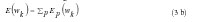
Mathematically it is denoted as

The Backpropagation algorithm in which the weights of the network are updated immediately after the presentation each pair of input and target output is called the sequential learning. The other learning procedure in which the whole training set is considered as a batch is called the batch learning. For sequential learning,

For batch-learning

Where, Ep(wk) denotes the mean squared error (MSE)for a pair of input and output. The learning or training process may be supervised, unsupervised or competitive. The aim of supervised learning is to find out a set of weight vectors that minimizes the deviation between network output and the target output over the whole training. The optimal weight matrix obtained this way is applied to the test set to investigate the viability of the model.

Data and analysis

Present paper deals with mean monthly total ozone concentration in Arosa, Switzerland between 1932 and 1971. The measurements are taken in Dobson Units (DU) (300 DU=1layer of 3mm if the whole ozone column is taken at the sea level with standard conditions). First of all, an autocorrelation analysis is performed on the dataset. The autocorrelation coefficients (for lag k) are computed as (Wilks, 1995)

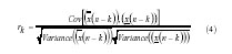
Where, r_k denotes the autocorrelation of order k,

denotes the first (n-k) data values,

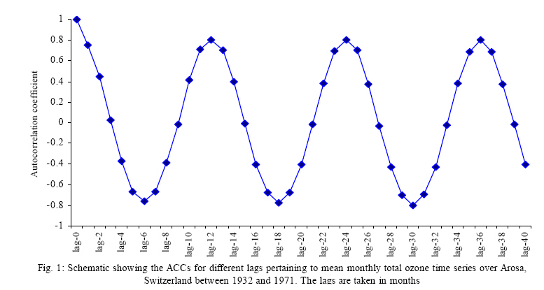
denotes the last (n-k) data values, and k varies from 1 to n. The autocorrelation coefficient (ACC) values are computed from the available data set up to 40 lags and their magnitudes are presented in Fig. 1. The Fig. makes it clear that the high ACC values are occurring at the lags 1,6,12,18 etc. That is, at lags separated by 5 time points. Thus, it can be inferred that mean monthly total ozone time series is completing a cyclic pattern in every 6 months. Thus, a predictive model can be developed with 5 months’data as predictor and the 6th month’s data as predictand.

Multiple linear regression model

A multiple linear regression model is proposed as

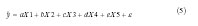
Where, the left hand side of equation (5) implies the predicted value of mean monthly total ozone in the 6th month with X1, X2, X3, X4 and X5 as predictors

i.e. the mean monthly total ozone in months 1,2,3,4 and 5. The constants a, b, c, d and e are the regression parameters computed by the method of least squares (Wilks, 1995). In the present study the regression equation comes out to be

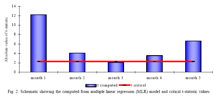
From this linear multiple regression fit it comes out that the coefficient of determination is 0.7512, which is not very far from 1. Thus, this linear fit is not a very bad predictive model. The values of tstatistic are computed from this model and are compared to the critical t-statistic value. The comparison is presented in Fig. 2, which shows that only the value of the time series in month 3 falls just below the critical value. Thus, it can be said that mean monthly total ozone concentration in the month t, depend heavily upon the values in the months t-5, t-4, t-2 and t-1; but does not depend significantly upon the month t-3.

Single hidden layer ANN models

In the previous discussion it has been established the value corresponding to the month t-3 does not depend influence the month t very significantly. Since ANN models can work even with not-so-correlated predictors, all the values can be considered on the same foot while constructing single-hidden-layer ANN models. In this paper, seventeen single-hidden-layer ANN models have been developed with Backpropagation algorithm explained in equation (1) through (3b). The models have been denoted as H1, H2, H3, H4, H5, H6, H7, H8, H9, H10, H11, H12, H13, H14, H15, and H16and H17. Here Hi implies that the model contains "i" number of nodes in the hidden layer. All the models have been trained separately with sigmoidal activation function up to 500 epochs sequentially with the aim that the mean squared error (equation (3b)) is to be minimized. From each input set, 75% data are considered as the training data and the remaining 255 data are considered as the test or validation data. To say more specifically, 120 data have been considered as validation set and 355 data are considered as training set. While training, learning rate has been taken as 0.9 and momentum rate has been taken as 0.2.

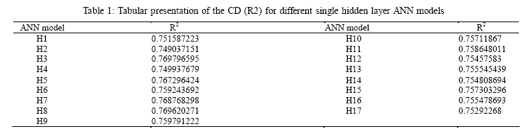
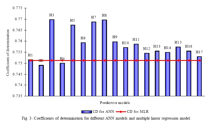
First of all, coefficients of determination conventionally denoted as R2 (Comrie, 1997) are computed for all the predictive models. It has been mentioned earlier that R2 for multiple linear regression (MLR) model is 0.7512. Now, R2 are computed for all the 17 ANN models and are presented in tabular form in Table 1. To compare the performance of different ANN models between themselves and with MLR model, Fig. 3 is prepared. This Fig. shows that all the ANN models excepting H2 and H4 produce higher CD than MLR model. Thus, H2 and H4 are discarded from our discussion. From the rest of the models it is found that H1 produces almost the same CD as by MLR. Thus, a single hidden layer model with only one node does not produce any overwhelmingly better prediction than MLR.

Models H6, H9-H17 produce significantly better prediction than MLR but are distribute more or less regularly around an average value. It is very important to note that up to H8, addition of hidden nodes is producing significant changes in the CD, but after that the CDs did not vary drastically and all of them are significantly lower than that produced by H8. From here it can be inferred that after 8 hidden nodes, adding more hidden nodes does not create any room for further improvement in the prediction. 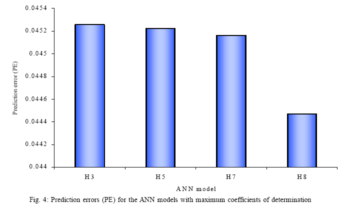The best CDs are produced by H3, H5, H7 and H8. The next task is to identify the best model among these four. Now, the prediction error (PE) (Perez and Reyes, 2001) over the whole test set are computed for each of the four models mentioned above and are schematically presented in Fig. 4. This Fig. clearly shows that the least PE is being produced by H8. From here it can be said that H8 is the best ANN model to forecast the mean monthly total ozone concentration over Arosa, Switzerland. 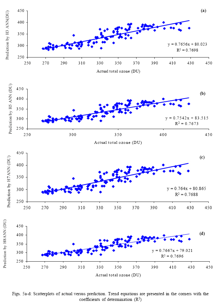But, to reach the final conclusion some qualitative tests are being executed. Scatter plots for the actual and predicted values corresponding to H3, H5, H7 and H8 are presented in Fig. 5a-d. The least square regression fits to the models are also presented in the Figs. It is apparent from those equations that the least y-intercept (79.021) by the trend equation occurs for H8. The other y-intercept values are 80.023 (H3), 83.515 (H5) and 80.865 (H7). 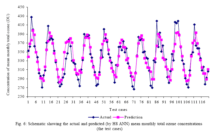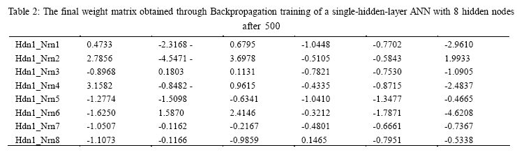Since for highest correlation between actual and prediction the y-intercept becomes 0, thus, the lowest y-intercept producing model (H8) can be considered as the best predictive model. After all these tests, H8 is identified as the best predictive model and the prediction by this model with the actual values are presented in Fig. 6. A very close association between the actual and the prediction can be viewed from here. The structure of the final model (H8) is presented in Table 2.

The rigorous study executed above leads us to conclude some important characteristics of the time series pertaining to total ozone time series over Arosa, Switzerland. The autocorrelation study reveals that mean monthly total ozone concentration over Arosa, Switzerland follows a cyclic pattern with 6 months cycle. Furthermore, the third month within the cycle has less significant impact upon the sixth month. Artificial Neural Network with Backpropagation learning has been established to be a potent predictive tool for the said time series. A comparative study with respect to prediction ability reveals that single hidden layer predicts the mean monthly total ozone concentration over Arosa, Switzerland more efficiently than multiple nodes is the best predictive model to forecast the mean linear regression model. A further comparative study monthly total ozone concentration over Arosa using among different neural net models proves that single-the past data values.

REFERENCES

• Balaguer Ballester, E., Valls, G., Carrasco-Rodriguez, J., Soria Oliva, E., Valle-Tascon, S., (2002). Effective 1-day ahead prediction of hourly surface ozone concentrations in eastern Spain using linear models and neural networks. Ecologic. Model., 156, 27-41.
• Corani, G., (2005). Air quality prediction in Milan: feed-forward neural networks, pruned neural networks and lazy learning, Ecologic. Model., 185, 513-529.
• Gardner, M.W., Dorling, S.R., (1998). Artificial Neural Network (Multilayer Perceptron)-a review of applications in atmospheric sciences. Atmos. Environ., 32, 2627-2636.
• Hsieh, W.W., Tang, T., (1998). Applying Neural Network Models to prediction and data analysis in meteorology and oceanography. Bulletin of the American Meteorological Society, 79, 1855-1869.
• Kartalopoulos, S.V., (2000). Understanding Neural Networks and Fuzzy logic-basic concepts and applications, Prentice Hall, New-Delhi
• Kamarthi, S.V., Pittner, S., (1999). Accelerating neural network training using weight extrapolation. Neur. Net., 12, 12851299.
• Maqsood, I., Muhammad, R.K., Abraham, A., (2002). Neurocomputing based Canadian weather analysis. computational intelligence and applications. Dynamic Publishers Inc., USA, 39-44.
• Milionis, A.E., Davis, T.D., (1994). Regression and stochastic models for air pollution, Part I: review comments and suggestions. Atmos. Environ., 28 (17), 2801-2810.
• Nunnari, G., Nucifora, M., Randieri, C., (1998). The application of neural techniques to the modelling of time-series of atmospheric pollution data. Ecologic. Model., 111, 187-205.
• Prybutok, R., Junsub, Y., Mitchell, D., (2000). Comparison of neural network models with ARIMA and regression models for prediction of Houston’s daily maximum ozone concentrations. Euro. J. Operat. Res., 122, 31-40.
• Shi, J.P., Harrison, R.M., (1997). Regression modeling of hourly NOx and NO2 concentration in urban air in London. Atmos. Environ., 31 (24), 4081-4094.
• Viotti, P., Liuti, G., Di Genova, P., (2002). Atmospheric urban pollution: application of an artifical neural network to the city of Perugia. Ecologic. Model., 148, 27-46.
• Wilks, D. S., (1995). Statistical methods in atmospheric sciences, Academic Press, USA

© 2007 Center for Environment and Energy Research and Studies (CEERS)

The following images related to this document are available:

Photo images