International Journal of Environment Science and Technology Center for Environment and Energy Research and Studies (CEERS) ISSN: 1735-1472 EISSN: 1735-2630 Vol. 4, Num. 2, 2007, pp. 215-222

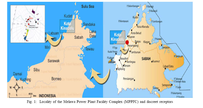
International Journal of Enviornmental Science and Technology, Vol. 4, No. 2, Spring 2007, pp.215-222

Computer simulated versus observed NO₂ and SO₂ emitted from elevated point source complex

^1*W.L. Freddy Kho, ²J. Sentian, ²M. Radojevic, ²C.L. Tan, ¹P.L. Law, ¹S. Halipah

¹Department of Civil Engineering, Universiti Malaysia Sarawak (UNIMAS) 94300 Kota Samarahan, Sarawak, Malaysia
²School of Science and Technology, Universiti Malaysia Sabah (UMS) Locked Bag No. 2073, 88999 Kota Kinabalu, Sabah, Malaysia
*Corresponding author, Email: frexwl@gmail.com Tel.: +6082-456877; Fax: +6082-456577

Received 4 August 2006;
Revised 25 February 2007;
Accepted 6 March 2007;
Available online 20 March 2007

Code Number: st07028

ABSTRACT: ISC-AERMOD dispersion model was used to predict air dispersion plumes from an diesel power plant complex. Emissions of NO₂ and SO₂ from stacks (5 numbers) and a waste oil incinerator were studied to evaluate the pollutant dispersion patterns and the risk of nearby population. Emission source strengths from the individual point sources were also evaluated to determine the sources of significant attribution. Results demonstrated the dispersions of pollutants were influenced by the dominant easterly wind direction with the cumulative maximum ground level concentrations of 589.86 µg/m³ (1 h TWA NO₂) and 479.26 µg/m³ (1 h TWA SO₂). Model performance evaluation by comparing the predicted concentrations with observed values at ten locations for the individual air pollutants using rigorous statistical procedures were found to be in good agreement. Among all the emission sources within the facility complex, SESB-Power (diesel power plant) had been singled out as a significant source of emission that contributed >85% of the total pollutants emitted.

Key words: ISC-AERMOD, plumes, diesel-fired, power plant complex, emission, stacks

Significant emissions of air pollutants, particularly in industrialised areas have always been a concern to in plant workers and nearby population in terms of air quality management. This is mainly due to the complexity of emissions sources, load of emissions, and type of emissions, variability of the local meteorological and terrain conditions as well as the presence of sensitive receptors in the surroundings of the air pollution sources. Air dispersion models (ADM) have been widely used to investigate the dispersion patterns and behaviour of air emissions in such areas (Mehdizadeh and Rifai, 2004), and also to assess the potential hazards to the human health (Zhou, et al., 2003; James, et al., 1995). ADMs are also used in air quality impact assessment on specific industrial facilities or a group of industry to assess the cumulative impact on the downwind pollutant concentrations and to predict future air quality in the surrounding for environmental management planning purposes. They are also used as a tool in environmental auditing exercises on the assessment audit of air quality impact as well as on the air pollution control efficiency on specific facilities. The model generated results could facilitate the respective authorities to make appropriate actions in accordance to the requirements of the relevant environmental laws and regulations. Point source emissions from various industrial sources have been the target for investigating the pollutants dispersion pattern by using various types ofADMs. For example, in power plants emission, ADMS 3.1 dispersion model had been used to model the dispersion of SO₂ (Carruthers, et al., 1997; Bennet and Hunter, 1997; Carslaw and Beevers, 2002), ISCST3 dispersion model for CO and NO _x (Venegas and Mazzeo, 2005), and CALPUFF dispersion model for PM_2.5 and other gases (Zhou, et al., 2003). Air dispersion model such as SCREEN was also used to study the dispersion of VOCs from various types of industries and their impact to the surrounding residential areas (James, et al., 1995).

Locality of study area

The objectives of this studywereto model or predict the maximum ground level concentrations of SO₂ and NO₂ emitted from Melawa Power Plant Facility Complex (MPPFC) as shown in Fig. 1 in order to assess the cumulative impact of emission to the surrounding environment using ISC-AERMOD View. Potential impact of pollutants exposure on selected discrete receptors within the 2 km x 2 km domain coverage was also assessed. The study also sought to determine the pollutants sources strength from emission sources within the MPPFC. MPPFC (latitude 6° 8’N; longitude 116° 13’E) is located within the Kota Kinabalu Industrial Park (KKIP). KKIP is an area established by the State Government for development of various types of industrial activities ranging from light to heavy industries, housing, commercial, institutions and conservation areas. As the development of KKIP area is still at its early stage, currently the only significant stationary source of air pollutants in this area is from the MPPFC. The MPPFC comprises of two power plants (SESB-Power and ARL-Power) and a waste oil incinerator (ARL-Incinerator). The facility is located on a 4.4-hactare land with elevation at approximately 15 meters above mean sea level. It is located about 23 km northeast of Kota Kinabalu City centre. The MPPFC is surrounded by industrial complexes on the east, and residential houses and institutions on the west, north and south (Fig. 1). Within the domain coverage of 3 km by 3 km, the topography is generally flat with ridges ranging from 5 m to 100 m in elevation.

Description of dispersion model

ISC-AERMOD View is the latest version of ISC models (Industrial Source Complex). It is a complete and powerful air dispersion modelling package which seamlessly incorporates the popular United States Environmental ProtectionAgency(USEPA)models into one interface: ISCST3, ISC-PRIME, AERMOD and AERMOD-PRIME. ISC-AERMOD view has incorporated the Plume Rise Model Enhancements (PRIME) building downwash algorithms, which provide a more realistic handling of downwash effects than previous approaches (MEO, 2003). PRIME model was designed to incorporate two fundamentals features associated with building wash which are (a) the enhanced plume coefficients due to the turbulent wake, and (b) the reduced plume rise caused by combination of the descending streamlines in the lees of buildings and the enlarged entrainments in the wakes. ISCAERMOD packaged is supported by Building Profile Input Program (BPIP) View which is a graphical user interface designed to speed up the work involved in setting up input data for the BPIP. BPIP was used to perform building downwash analysis for point sources in order to run the model. Data input for location and dimension of buildings (structures) and stacks can be done either by graphic, where the buildings and stacks can be digitised on the screen with the mouse, or by text mode, where information can be added in a spreadsheet-like input form.

ISC-AERMOD View has also incorporated essential user-friendly options such as complete RAMMET and AERMET meteorological data pre-processing and multiple pollutant utilities for modelling multiple pollutants in a single ISCST3, ISC-PRIME or AERMOD run (Jesse, et al., 2000). The AERMET program is a meteorological pre-processor, which prepares hourly surface data and upper air data in the modelling. AERMET processes meteorological data in three stages. Firstly, the meteorological data extracted from archive data files and processed the data through various quality assessment checks. Secondly, all the available data for 24 h. periods were merged and stored in a single file. Lastly, the merged data was read and boundary layer parameters were estimated for use in the AERMOD model. Wind rose was also plotted using WRPLOT View based on the analysed meteorological data.

The ISC-AERMOD View interface uses six pathways that compose the run stream file as the basis for its functional organization (Jesse, et al., 2000). These pathways are:

• Control Pathway (CO): Where the modelling scenario is specified, and control of the overall modelling run;
• Source Pathway (SO): Where the sources of pollutant emissions are defined;
• Receptor Pathway (RE): Where the air quality impacts on specific receptors locations are defined;
• Meteorological Pathway (ME): Where the atmospheric conditions of the area being modelled are defined;
• Terrain Grid Pathway (TG): Where the option of specifying gridded terrain data to be used in calculating dry deposition in elevated or complex terrain is available, and
• Output Pathway (OU): Where the output results are defined.

Data acquisition Meteorological data

The meteorological parameters data input for this modelling were obtained from the surface weather observatory station at Kota Kinabalu International Airport located 40 km south of the MPPFC. A detailed analysis of the meteorological data such as ceiling height, wind speed, wind direction, air temperature, total cloud opacity and total cloud amount has been made over five years (1996-2001). The dominant wind direction was of easterly wind. The wind speed was in the range between 1.3 and 3.6 m/s with an average of 1.97 m/s. A multi-directional wind was taken into account for this study to calculate the overall dispersion of pollutant concentration surrounding the point sources area. About 35.5% of the time, this easterly wind speed was within the range between 0.5 m/s and 3.6 m/s. Referring to the annual 24 h wind direction, the frequencies of other wind directions were all below 10%. In determining atmospheric stability, Turner’s StabilityClassification Method was used. In this study, for short time periods, atmospheric stability of the atmosphere was assumed to be constant and based on the mean velocity of the wind speed, the atmospheric stability of Class B was chosen which is defined to be moderately not stable. Movement of air in the vertical dimension is enhanced by vertical temperature differences. The steeper the temperature gradient is, the more vigorous the convective and turbulent mixing of the atmosphere. The larger the vertical column in which turbulent mixing occurs, the more effective the dispersion process, which is defined by the mixing height. Mixing height used in this study was 1,000 m.

Building and stack data

For modelling purposes, the physical and emission data of each stack within the MPPFC site were obtained from the database supply by MPPFC operators. Location and dimension of stack, building and any major structure within the complex were also obtained as an input for BPIP in calculating and analysing the building downwash effects. BPIP data input for location and dimension of buildings (structures) and stacks can be done either digitising graphically on the screen or adding structures information in a spreadsheet. Table 1 summarises the operational characteristics and stack and emission properties of the MPPFC.

Air quality monitoring

The current status of air quality within the study domain was determined by on site ground level measurement. Ground level measurements of pollutants at ten sites within the domain coverage were established. The ground level monitoring sites (R1R10) are situated at strategic locations mainly in residential areas as well as institutional and industrial sites as shown in Fig. 1. The monitoring sites were also identified as discrete receptors locations. The ground level concentrations data of pollutants were used to validate the predicted value from the emission modelling. Table 2 summarises the ground level pollutant measurements, instrumentation and operational specifications.

Receptors information

In evaluating the exposure of pollutants emission from the MPPFC to the surrounding population, ten discrete receptors (R1-R13) were selected within the study area (Fig. 1). Most of the receptors are residential and institutional areas (Table 2). In assessing the potential impact on public health, the predicted values were compared with/to the Malaysian Ambient Air Quality Guideline Standard (DOE Malaysia, 2000) for the respective pollutants.

Model performance criteria

The applications of rigorous statistical procedures (Hanna, 1989; Kumar, et al., 1999) were used to quantitatively evaluate the performance of the model. Generally, the model would be considered acceptable if it meets the following performance criteria:

(a) Fractional Bias (FB) which is the mean error that defines the residual of the observed and the predicted concentrations. It has the value of zero for an ideal model and varies between -2 and 2 and express as:

FB = (o>-p>)/0.5(o+p>)

Where C_o is observed concentrations and C_p is predicted concentrations. Note that a < > bracket indicates an average over all points in the group. The model is considered acceptable when, -0.5d”FBd”0.5.

(b) Normalized mean square error (NMSE) which emphasizes on the scatter of the entire data set. Zero value of NMSE indicates an ideal model performance. It is express as:

NMSE = < (C_o-C_p)²>)/ (o>p>)

Where C_o is the observed concentrations and C_p is the predicted concentrations. Note that a < > bracket indicates an average over all points in the group. The model is considered acceptable when, NMSE d”0.5.

(c) Factor of 2 (FAC2) which is the percentage of predictions, where the predictions and observed values are within a factor of 2 from one another (0.5d” (C_p/ C_o)d”2). The model is considered acceptable when, FAC2³ 0.8.

Table 1: Operational characteristics, stack and emission properties

Table 2: Receptors identification within the domain coverage

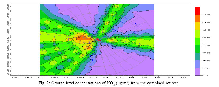
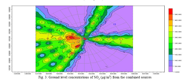
RESULTS

Cumulative and individual impacts assessment

Cumulative impact on ground level concentrations of pollutants, emitted from combined sources was modelled and the results are depicted in Figs. 2 and 3. Similar dispersion patterns were also observed for individual source (SESB-Power, ARL-Power and ARLIncinerator) but with varied ground level concentrations as shown in Table 3. Based on worse-case scenario, where both power plants and incinerator were in operation, the predicted maximum 1 h averaging ground level concentration of NO2 was 613.851μg/m³ , which was observed at approximate distance of 1.0 km to the southwest (coordinate x-430312.72, y-5299302.00). Maximum ground level concentration of SO₂ was also observed at approximately similar distance and direction of that NO₂ , which was 554.48 μg/m³ (coordinate x– 430312.72, y – 5299302.00). The ground level concentrations of the pollutants at receptors in residential/villages and institutional areas are shown in Table 3. During the study period, the SESB-Power wasnot in operation (note: the power plant was not fully inoperation since a year ago due to technical and economic reasons). Based on the current scenario (without SESBPower), the ground level concentrations were expected primarily from ARL-Power with some attribution from ARL-Incinerator. Potential health impact on receptors was assessed by comparing the predicted ground level concentrations with/to the Malaysian Ambient Air Quality Guideline (DOE Malaysia, 2000). Based on the worse scenario receptors such as Tmn Sapangar (R9), KK Politeknik (R6) and Kg. Salut (R4) were exposed to high concentration of NO₂ , which exceeded the limit of 320 μg/m³ (1h, TWA).

SO₂ was also observed to exceed the limit of 350 μg/ m3 (1h, TWA) at Kg. Malawa/Tmn Sapangar. However, considering that the SESB-Power was not in operation during the study time, the ground level concentrations of NO2 and SO2 at all receptors observed were well below the allowable limits. Based on the current scenario, ground level pollutant concentrations would not impose any significant impact to the nearby area.

Table 3: Ground level concentration of pollutants at selected receptors from individual and combined sources

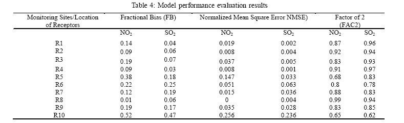
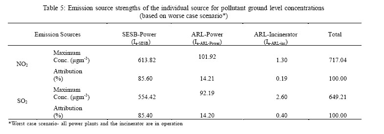
Model performance evaluation

To evaluate the performance of the model, the concentrations of the observed and predicted pollutants were statistically measured and the results of the model performance analysis are presented in Table 4. Based on the Fractional Bias (FB) values, the performance of the model for NO₂ and SO₂ at each monitoring sites/receptors location were within the acceptable ranges (-0.5d”FBd”0.5) except for NO₂ at R10. Performancemeasuresin term ofNormalised Mean Square Error (NMSE) were also found to be satisfying the criteria (d”0.5). The results showed reasonably good agreement between the predicted and observed values. Meanwhile, the performance measurements were based on Factor of 2 (FAC2) with more than 90% of the hourly average values within a factor of two (with ≥0.8). Three locations namely, R10 (for NO₂ and SO₂) and R5 (for NO₂) were observed to have less than the acceptable limit of ≥0.8, but still within a factor of two. Traffic emissions particularly NO₂ could partly attribute this result.

Emission source strengths

This study was also aimed to identify the emission source strength of each source of emission within the MPPFC. Relative emission-source strength has been determined at locations where recorded maximum ground level concentrations of pollutants by calculating the percentage of attribution.Table 5 shows the attribution of each source to the ground level concentrations. Based on worse-case scenario, it had been observed that SESB-Power has attributed more than 85% of ground level concentration of NO₂ and SO₂. Meanwhile the emission attributions from ARL-Power and ARL-Incinerator for all pollutants were generallyless than 15%.Apart from the characteristics of the emission load of pollutants from the SESB-Power, which are relatively higher, other possible explanation could be due to the building downwash effect. The heights of the three stacks of SESB-Power are relatively shorter (9 m) thanthe height ofthe power plant building (20 m). Buildings and other structures near a relatively short stack can have a substantial effect on plume transport and dispersion, and on the resulting ground level concentrations that are observed. The stack height factor has induced the occurrence of building downwash phenomena within the facility complex, which had drawing the plume to the ground near the source (Venkatram, et al., 2004).When the airflow meets power plant building, it is forced up and over the building. On the lee side of the building, the flow separates leaving a closed circulation containing lower wind speeds. Farther downwind, the turbulent wake zone was created where the airflow forced downward again and in addition with the creation of shear, which induced more turbulence. The plume emissions from the SESB-Power most likely caught in the cavity and if the plume escaped the cavity, but remains in the turbulent wake, it may be carried downward and dispersed more rapidly by the turbulence. This condition could result in either higher or lower concentrations than would occur without the building. It is depending on whether the reduced stacks height or increased turbulent diffusion has the greater effect. In minimising the building downwash effect installation of at least twice the height of adjacent building as the operating rule should be sufficient to minimise the effect of building downwash (Wark, et al., 1998), or application of good engineering practice of stack height (MEO, 2003). The higher stacks enabled pollution to be dispersed away from the source areas competently compare to the shorter stacks (Downer and Radojevic, 1992).

DISCUSSION AND CONCLUSION

This study has focused on ground level observations and modelling analyses of NO₂ and SO₂ dispersion from various elevated point sources within the MPPFC in elucidating pollutants dispersion patterns, emission source strengths and emission potential risks on selected receptors within the domain coverage. Modelling analysis using ISC AERMOD View showed that the two pollutants were dispersed dominantly to the west in corresponding with the easterlydominant wind direction. Small fractions were also dispersed to the east and north directions. Analysis on the emission source strengths showed that emission from SESB-Power has attributed to the emission of more than 85% of NO₂ and SO₂. This suggests that SESB-Power had significantly attributed to the ground level concentration of pollutants in the study area. One of the main factors that could lead to this result was the height of the stacks, which were found to be shorter and not conformed to the stack height requirement. This condition has allowed the building downwash phenomena to occur which had drawing the plume to the ground near the source. A total number of discrete receptors, mainly residential area within the domain coverage were assessed in terms of exposure to air pollutants by comparing with the Malaysian Ambient Air Quality Standard Guidelines. The computer simulated results based on worse case scenario showed that receptors such as Kg. Malawa/Tmn Sapangar (R9), KK Politeknik (R6) and Kg. Salut (R4) were exposed to high concentration of NO₂, which exceeded the limit of 320 µg/m³ (1h, TWA). SO₂ was also observed to exceed the limit of 350 µg/m³(1h, TWA) at Kg. Malawa/Tmn Sapangar. However, by considering that the SESB-Power was not in operation during the study period, the ground level concentrations of NO₂ and SO₂ at all receptors were observed to be well below the allowable limits. Based on the current scenario, the pollutants ground level concentrations would not impose any significant impact to the surrounding area.

REFERENCES

• Bennet, M., Hunter, G.C., (1997). Some comparisons of Lidar estimates of peak ground-level concentrations with the predictions of UK-ADMS, Atmos. Environ., 31 (2), 429-439.
• Carruthers, D.J., Edmunds, H.A., Bennet, M., Wood, P.T., Milton, M.J.T., Robinson, R., Underwood, B.Y., Franklin, C.J., Timmis R., (1997). Validation of the ADMS dispersion model and assessment of its performance relative to R-91 and ISC using archived LIDAR data. Int. J. Environ. Pollut., 8 (3-6), 264-278.
• Carslaw, D.C., Beevers S.D., (2002). Dispersion modelling concentrations for transient emissions from elevated point sources, Atmos. Environ., 36, 3021-3029.
• Department of Environment Malaysia. (2000), A Guide To Air Pollution Index I Malaysia, Ministry of Science, Technology and Environment, Kuala Lumpur.
• Downer, R.M., Radojevic, M., (1992). Technologies of Control, in Atmospheric Acidity, Eds. M. Radojevic, R.M. Harrison, Elsevier Science Publishers Ltd, U.K., 467-494.
• Hanna, S.R., (1989). Confidence limits for air quality model evaluations as estimated by bootstrap and jackknife resampling methods, Atmos. Environ., 23, 1385-1398.
• James, K.J., Cherry, M., Stack, M.A., (1995), Assessment of chemical plant emission on an urban environment: A new approach to air quality measurements, Chemosphere, 31, (7), 3741-3751.
• Jesse, L., Cristiane L., Michael A., (2000). User’s Guide ISCAERMOD View, Volume I & Volume II, Lakes Environmental Pt. Ltd., Ontario, Canada.
• Mehdizadeh, F., Rifai H.S., (2004). Modelling point source plumes at high altitudes using a modified Gaussian model, Atmos. Environ., 38, 821-831.
• Ministry of Environment Ontario (MEO), (2003). Proposed guidance for air dispersion modelling [online]. Ministry of Environment Ontario. Available from http:// www.ene.gov.on.ca/envision/techdocs/3614e02.pdf>
• Kumar, A., Bellman N.K., Sud A., (1999). Performance of an industrial source complex model: predicting long-term concentrations in an urban area. Environ. Prog., 18(2). 93-100.
• Mazzeo, N.A., Venegas, L.E., (2000). Practical use of the ISCST3 model to select monitoring site locations for air pollution control. Int. J. Environ. Pollut., 14 (2), 1-6.
• Rama Krishna, T.V.B.P.S, Reddy, M.K., Reddy, R.C., Singh, R.N., (2004). Assimilative capacity and dispersion of pollutants due to industrial sources in Visakhapatnam bowl area. Atmos. Environ., 38, 6775-6787.
• Venegas, L.E., Mazzeo, N.A., (2005). Modelling of urban background pollution in Buenos Aires City (Argentina). Environmental Modelling & Software.
• Venkatram, A., Isakov, V., Yuan, J., Pankratz, D., (2004). Modeling dispersion at distances of meters from urban sources. Atmos. Environ., 38, 4633-4641.
• Wark, K., Warner, F.C., Davis, T.W., (1998), Air Pollution. Its Origin and Control, 3^rd. Ed. Addision-Wesley, Longman.Inc.
• Yassin, M.F., Kato, S., Ooka, R., Takahashi, T., Kouno R., (2003). Study on effects of fluctuations in the wind direction on pollutant diffusion in urban areas. in Proceedings of the 11^th. International Conference on Modeling, Monitoring and Management of Air Pollution, Eds. C.A. Brebbia & F. Patana, WIT Press, U.K., pp 143-151.
• Zhou, Y., Levy, J.I., Hammitt, J.K., Evans, J.S., (2003). Estimating population exposure to power plant emissions using CALPUFF: A case study in Beijing, China. Atmos. Environ., 37, 815-826.

© 2007 Center for Environment and Energy Research and Studies (CEERS)

The following images related to this document are available:

Photo images