International Journal of Environment Science and Technology Center for Environment and Energy Research and Studies (CEERS) ISSN: 1735-1472 EISSN: 1735-2630 Vol. 5, Num. 3, 2008, pp. 323-330

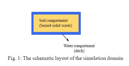
International Journal of Enviornmental Science and Technology, Vol. 5, No. 3, Summer 2008, pp. 323-330

Transient and spatial modeling and simulation of polybrominated diphenyl ethers reaction and transport in air, water and soil

^1* M. Mousavi; ¹ S. Kiani; ² S. Lotfi; ³ N. Naeemi; ¹ M. Honarmand

¹ Department of Chemical Engineering, Faculty of Engineering, Ferdowsi University of Mashhad, Mashhad, Iran
² Materials and Energy Research Center, Karaj, Iran
³ Faculty of Chemical Engineering, Sahand University of Technology, Tabriz, Iran

Received 30 March 2008; revised 20 April 2008; accepted 8 May 2008; available online 1 June 2008

Code Number: st08037

ABSTRACT

The release of the wastes containing polybrominated diphenyl ethers into the environment is a worldwide major concern. Investigation of spatial and temporal variations of polybrominated diphenyl ethers concentrations due to different factors, especially the transport of these species between air and water as well as between air and soil is the purpose of present research. A model was developed and solved using the methods of finite difference and lines. Simulations were implemented for three dimensions of width, length, and height and also time for the air compartment, whereas for the soil and water compartments, variations were considered only with respect to height and time. Transport between water and soil was disregarded for simplicity at this stage. Vancouver's landfill was considered as a case study. Lower concentrations in air and higher concentrations in water at the interface show that these pollutants tend to diffuse from air to water. Concentrations of all four pollutants decrease near the interface in soil as time passes, but they are predicted to be almost constant at other levels.

Key words: Landfill, flame retardant, pollutant, model, finite difference, method of lines

INTRODUCTION

Flame retardants are added to polymeric materials to enhance their flame retardancy (Alaee et al., 2003). They can be divided into four families (Alaee and Wenning, 2002): inorganic flame retardants, halogenated flame retardants, organo-phosphorous flame retardants, and nitrogen-based organic flame retardants. Brominated flame retardants (BFRs) belong to the family of halogenated flame retardants (Arias, 1992, de Wit, 2002). Polybrominated diphenyl ethers (PBDEs) are the most stable BFRs, and they are found widely in the environment (Alaee et al., 1999; KEMI, 1995). They are highly lipophilic, enabling significant bio-accumulation in animals and humans (Hale et al., 2003; McDonald, 2002). They are considered highly toxic, persistent, and bioaccumulative, with potential for long-range transport. They are regarded as potential Persistent Organic Pollutants (POPs) (Webster et al., 1998). However, under a 2001 agreement signed in Estockholm, PBDEs must be controlled globally because of their severe threat to human lives and the environment (Rayne et al., 2003; Wenning, 2002).

Although there are four commercial PBDE products i.e. tetra-, penta-, octa-, and deca-BDE in old PBDE-containing wastes, each is composed of congener mixtures. Incidentally there has been a shift in use toward the higher brominated compounds especially deca-BDE recently (Alaee et al., 2003; Darnerud et al., 2001). Industry uses these compounds because of their low cost, thermal stability and the efficiency which the halogen atoms chemically reduce and retard fire (Darnerud et al., 2001). PBDEs are chemically synthesized and have been used in electrical and electronic supplies such as covers of wires and cables, linkages and printed circuit boards (de Boer et al., 2000). They may also constitute up to 30% of such products as computers, television sets, and upholstery (Alaee et al., 2003, Hedelmalm et al., 1995).

Although many manufacturers either have substituted or will soon replace some BFRs in electronic equipment, older models known to contain substantial quantities of BFRs are now entering the disposal or end-of-useful-life phase. Disposal in landfills is one of the most important elimination methods of this obsolete equipment. There is concern with respect to their release into the environment from landfills, especially by leaching (Osako et al., 2004). This leachate may cause water pollution. Moreover, evaporation from these landfills and gases produced from incineration of wastes containing PBDEs yields air pollution. The deposition of these pollutants on plants or the transmission of them to plants via water causes pollution in plants. Some PBDEs are persistent in the environment. Therefore, long-term diffuse emissions from landfills may also be problematic (Danish EPA, 1999). As their pollution is significant in all environmental parts and they are persistent, toxic and bio-accumulative, PBDEs have attracted global concern, requiring experimental and modeling/simulation research. Current approaches to modeling the formation and transportation of persistent organic pollutants (POPs) in the environment have evolved in response to four dominant types of models (Wania et al., 1999):

1. models describing specific processes (e.g. air-to-surface exchange);
2. models evaluating and assessing generic chemical fate (e.g. models used to evaluate general environmental behaviour and classification of chemicals);
3. models describing biological uptake;
4. models describing actual chemical fate on a local, regional and global scale (e.g. a lake, river or region).

Multi-compartmental models, which describe actual chemical fate, are from type 4. These models account for compartments such as air, water and soil. They have had significant development. Early models were either based on equilibrium or neglected time changes. Also decomposition reactions of materials and their transport were ignored. These models are based on fugacity. In the latest model, the system is neither at equilibrium nor steady. It accounts for transport processes and decomposition reactions (Mackay et al., 1996). here has been no mass transfer model accounting for landfills in which electric and electronic instrumentations and supplies containing flame retardant materials such as PBDEs are buried. Since these materials are transported among media such as air, water, and soil, their spatial and transient multi-compartmental modeling and simulation in three compartments of air, water, and soil simultaneously, which is the main purpose of the present paper, is complex. Considering spatial or dimensional variations is a new and complicated item of present modeling.

MATERIALS AND METHODS

The purpose of present modeling is to investigate spatial and temporal variations of species concentration due to different factors especially species transport between air and water, as well as between air and soil. Because transport of components between water and soil is disregarded, only the vertical direction is considered for modeling of water and soil at this stage. For air, however, the model equations are developed in all three directions. The component continuity equation for air is:

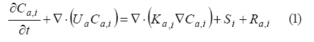
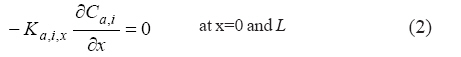
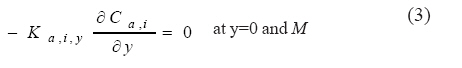
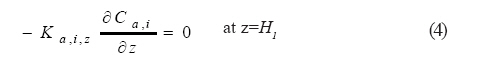
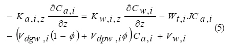
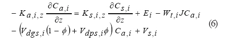
where subscript i refers to i^th component, is the concentration in atmosphere, t denotes time, U_a is the wind velocity, K_a is the diffusivity in the atmosphere, S is the rate of production (or destruction if negative) and R_a is the reaction rate. One needs six boundary conditions. Eqs. 2 to 6 are the boundary conditions in the x, y, and z directions for Eq. 1, with Eq. 5 applying between air and water and Eq. (6) between air and soil.

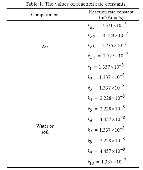
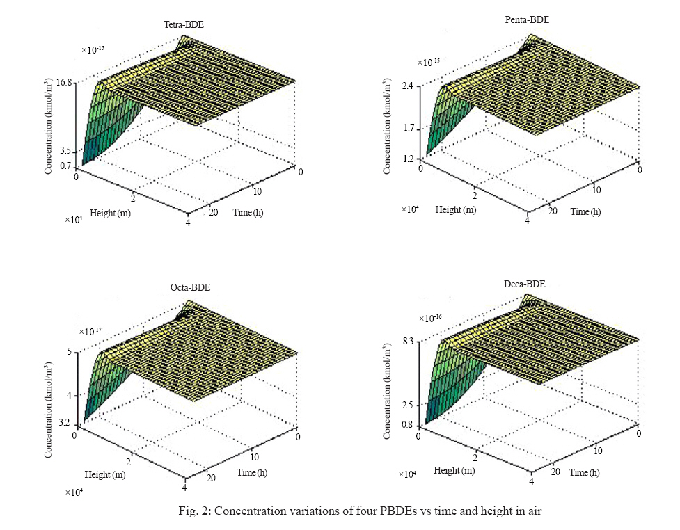
Here L, M, and H₁ are atmospheric dimensions of the modeling region, K_w is the diffusivity in water, C_w is the concentration in water, V_dgw is the dry deposition velocity from the gas phase of the atmosphere to water, V_dpw is the dry deposition velocity from the particle phase of the atmosphere to water, and V_w is the volatilization rate from water. The corresponding parameters for soil appear in Eq. 6. W_t, J, and E are total washout ratio, precipitation rate, particle-associated fraction of the component, and emission rate from sources at ground level respectively. W_t is related to W_g and W_p, the washout ratios of gas and particle phases, (Atkinson, 1996) by:

The initial condition for Eq. 1 is given by:

C _{a ,i} = C _{a ,i ,o} (8)

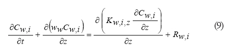
in which C_{a, i, o} is the initial concentration of species i in the atmosphere.

The main governing equation of the water compartment and its boundary condition at the air-water interface are:

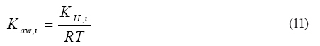
C _{a ,i} = K _{a w,i}C_w, (10)

where W_w is the vertical velocity of water, R_w is the reaction rate in water, and K_aw is the air-water partition coefficient. The last parameter is obtained using Eq. 11 (Scheringer, 1996):

in which K_H is the Henry's law constant, R is the universal gas constant, and T denotes temperature. The boundary condition at water depth H₂ and initial condition for Eq. 9 are similar to Eqs. 4 and 8, respectively. One can write similar equations for the soil compartment as for the water compartment, but with Eqs. 12 and 13 for calculation of K_as, the air-soil partition coefficient (Scheringer, 1996):

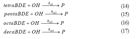
where

K _{sw ,i} = f _oc K _{oc ,i} = 0.41 f _oc K _{ow ,i} (13)

Here K_sw, K_oc and K_ow are the soil-water, organic mater-water, and octanol-water partition coefficients, respectively, and f_oc is the fraction of organic carbon in the soil. H₃, the soil depth, is taken as infinite.

PBDEs react with the hydroxyl (OH) in the atmosphere to form products (Totten et al., 2002):

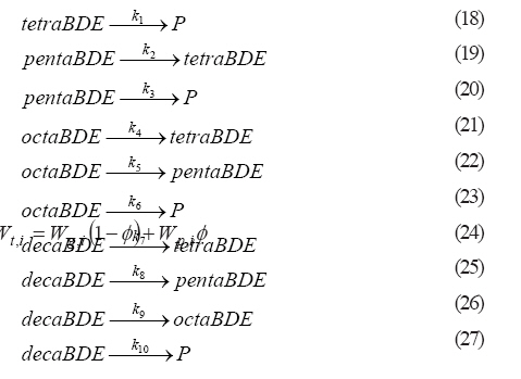
Assuming a steady-state concentration of the OH radical of 3×10⁶ molecules cm^-3 (Howard et al., 1991), the rate constants for reactions 14 to 17 correspond to half-lives of PBDEs.

PBDEs are debrominated to other PBDEs and products in soil and water (Kastanek et al., 1999):

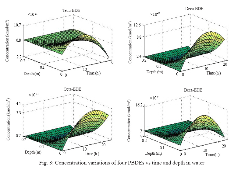
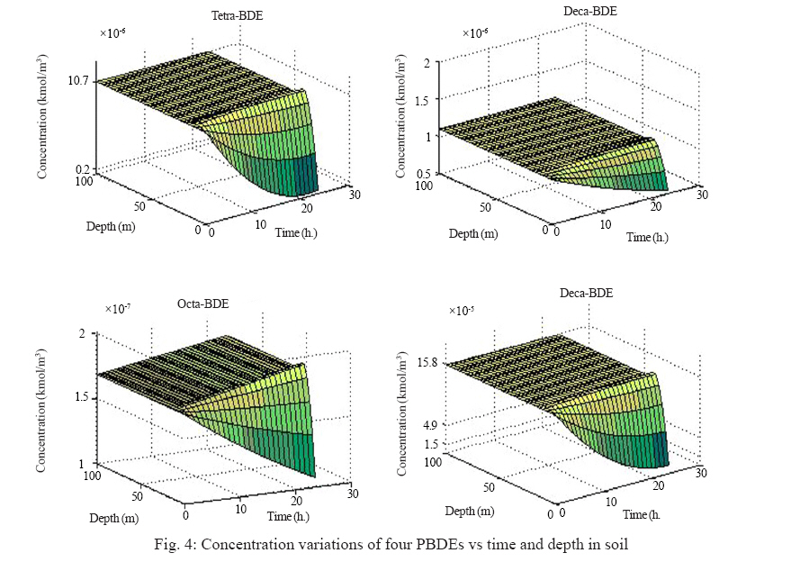
The rate constants for reactions 18 to 27 are estimated using the half-lives of PBDEs obtained from (Palm et al., 2002; Gouin and Harner, 2003).

The aim of the present simulation is to study the concentrations of four pollutants in three compartments soil, water, and air around a landfill in which wastes containing pollutants are piled. The simulation was implemented for three dimensions as well as time for the air compartment, but only for height and time for the soil and water compartments. The finite difference method and Method of Lines (MOL) were separately used to solve the model. The results were same with applying any two methods. MATLAB well known software was applied for simulation. Vancouver's landfill was considered as a case study. The landfill layout has been shown in Fig. 1. The height, length, and width of the landfill were taken as 4000 m, 3380 m and 820 m, respectively. Leachate flows in channels around the soil with a height of 0.2 m and a width of 2.3 m, respectively. The air is in contact with these two compartments. With respect to dimensions selected above and in order to converge to best results, the increments were defined. For height, length, and width in air compartment, 2000 m, 845 m and 205 m were selected respectively. For depth in water compartment 0.1 m and for depth in soil compartment 10 m was selected. And finally, an increment of 12 h. was selected for time in all three compartments.

The chemical, physical, and thermodynamic parameters as well as the meteorological parameters must be specified before simulation can be carried out. Temperature, average hourly wind velocity, average hourly angle of wind, and mixing layer length were obtained from the Canada's Meteorological Organization website. Vancouver's landfill office has supplied us with the characterizations of the landfill. The reference height was from Vancouver's weather station organization. Input data were obtained as follows: total suspended particles concentration, particle-gas partition coefficient (Ogura et al., 2003); dry deposition velocity of particle-phase chemical for soil and water, total washout ratio; estimated reaction rate constants for air , soil, and water (Palm et al., 2002, Gouin et al., 2003); solute molar volume at its normal boiling point (Palm et al., 2002); octanol/water partition coefficient and Henry's law constants for penta-, octa-, and deca-BDE (www.atsdr.cdc.gov); initial concentrations for water, soil, and air (Osako et al., 2004); octanol/water partition coefficient and Henry's law constant for tetra-BDE (www.nicnas.gov.au); roughness length (Arya, 2001); molecular mass for all four pollutants (Sweetman et al., 2004).The values of reaction rate constants have been represented in Table 1. The values of octanol-water partition coefficient of tetra-, penta-, octa-, and deca-BDE are 1×10^6.77, 1×10^6.57, 1×10^6.29, and 1×10^6.265 respectively.

After inserting the input data into the program, some related constants such as air/soil partition coefficient, vertical diffusivity for air, air latitudinal velocity were calculated. Some of these constants such as Richardson number must be obtained by trial and error. Next, the process of calculating concentrations for all times and places begins. For air, the reaction rate is calculated for all times and places, using initial concentrations and reaction rate constants. Time and location dependent equations which are influenced by parameters such as initial concentrations and reaction rate constants are then solved to obtain pollutants concentrations at all times and places in air compartment. Pollutant generation and consumption rates in air are assumed to be zero. Based on these assumptions, pollutant concentrations are calculated for the air-water and soil-air interface. A similar sequence is performed for the water compartment and then for the soil compartment to estimate pollutant concentrations for different times and heights.

RESULTS AND DISCUSSION

Data obtained from the program can be used to plot three-dimensional figures of concentration versus width-length and height-time.

Concentration changes of four pollutants in air in terms of time and height are shown in Fig. 2. The concentrations of all four pollutants increase with increasing height, finally reaching constant values. There is a decrease in pollutant concentrations during 24 h. due to reactions in this compartment. Concentration changes of four pollutants in air are essentially independent of the width and length coordinates. One can assume air as a homogenous compartment in which concentration changes only occur in its boundary layer. Furthermore, the concentration in air is only dependent on height and time. The lower concentrations at the interface show that these pollutants tend to be absorbed at the air-water interface. Concentration changes of four pollutants in water versus time and depth are shown in Fig. 3. Concentrations of these four PBDEs increase and then decrease near the interface with time due to the complex reactions and transport among the compartments. At greater depths, concentrations of tetra-, penta- and octa-BDE are predicted to increase a little with time, but deca-BDE concentration decreases a little as time passes. This is logical, since deca-BDE has no generation source and is being consumed by the reactions, whereas the other three pollutants have generation terms. This figure also shows a reduction in concentrations for all four pollutants with increasing depth. With higher concentrations at the interface in the water compartment, these pollutants tend to diffuse from air to the water compartment.

With respect to Fig. 4 related to the soil compartment, the concentrations of all four pollutants decrease as time passes near the interface. This is because of complex reactions and also transport among compartments. With regard to Fig. 4, the concentrations of tetra- and deca-BDE decrease a little, while the concentrations of the two other PBDEs increase a little as time passes in other places. Since deca-BDE is only being consumed, it is logical that its concentration deceases with time. Tetra-BDE is generated from the other PBDEs, but its decomposition rates are higher in soil, resulting in a reduction in its concentration, but not as much as deca-BDE. On the other hand, the generation rates are higher than the consumption rates for penta and octa-BDE and their concentrations increase. The concentrations of all four pollutants are almost independent of depth due to the higher concentrations of the four pollutants in this compartment relative to the other two compartments.

CONCLUSION

A model was developed in order to study the variations of polybrominated diphenyl ethers concentrations due to such factors as their transport between air-water as well as air-soil. Using finite differences, simulation was implemented for three compartments air, water, and soil. The results suggest that:

• Concentrations of all four PBDEs increase with height and decrease with time, showing negligible variation with length and width.
• Concentrations of the four pollutants in water are predicted to increase and then decrease near the interface with passing time, but follow a different pattern at greater depths. There is a reduction in concentrations with increasing depth. Lower concentrations in air and higher concentrations at the water in interface result from the diffusion of these pollutants from air to water.
• Concentrations of four PBDEs in soil are predicted to decrease with time near the interface, but they are almost constant at greater different depths.

Future research in this field should include length and width for water and soil compartments and different phases of these two compartments in the modeling and simulation.

ACKNOWLEDGEMENTS

The authors express their sincere appreciations to Prof. Grace, Prof. Elnashaie, and Dr. Danon-Schaffer in The University of British Columbia for scientific support.

REFERENCES

• Alaee, M.; Arias, P.; Sjödin, A.; Bergman, A., (2003). An overview of commercially used brominated flame retardants, their applications, their use patterns in different countries/regions and possible modes of release., Environ. Int., 29 (6), 683-689.
• Alaee, M.; Luross, J.; Sergeant, D.B.; Muir, D.C.G.; Whittle, D.M.; Solomon, K., (1999). Distributions of polybrominated diphenyl ethers in the Canadian Environment., Organohalogen Compd., 40 (3), 347-350.
• Alaee, M.; Wenning, R., (2002). The significance of brominated Flame retardants in the environment: Current understanding, issues and challenges., Chemosphere, 46 (5), 579-582.
• Arias, P., (1992). Brominated diphenyloxides as flame retardants: bromine based chemicals. Consultant Report to the OECD, Paris, France.
• Arya, S.P., (2001). Introduction to micrometeorology. Academic Press, San Diego.
• ATSDR, (2005). Toxicological profile for polybrominated biphenyls and polybrominated diphenyl ethers (PBBs and PBDEs). Chapter 6. Chemical and physical information. Publications of agency for toxic substances and disease registry, available at: http://www.atsdr.cdc.gov/toxprofiles /tp68-c6.pdf
• Atkinson, R., (1996). Atmospheric chemistry of PCBs, PCDDs and PCDFs. In: Hester, R. E.; Harrison, R. M., Eds., Chlorinated Organic Micropollutants. No. 6, Royal Society of Chemistry, Cambridge (UK).
• Danish EPA, (1999). Brominated Flame Retardants: Substance Flow Analysis and Assessment of Alternatives. Env. Project No. 494/1999.
• Darnerud, P. O.; Eriksen, G. S.; Jóhannesson, T.; Larsen, P. B.; Viluksela, M., (2001). Polybrominated diphenyl ethers: occurrence, dietary exposure and toxicology., Environ. Health Persp. Sup., 109 (S1), 49-68.
• de Boer, J.; de Boer, K.; Boon, J. P., (2000). Polybrominated biphenyls and diphenyl ethers. In: Paasivirta, J., Eds., The handbook of environmental chemistry, Vol. 3 Part K. New Types of Persistent Halogenated Compounds. Springer-Verlag Berlin Heidelberg.
• de Wit, C. Y., (2002). An overview of brominated flame retardants in the Environment., Chemosphere, 46 (5), 583-624.
• Gouin, T.; Harner, T., (2003). Modelling the environmental fate of the polybrominated diphenyl ethers., Environ. Int., 29 (6), 717-724.
• Hale, R.; Alaee, M.; Manchester-Neevig, J. B.; Stapleton, H. M.; Ikonomou, M. G., (2003). Polybrominated diphenyl flame retardants in the north American Environment., Environ. Int., 29 (6), 771-779.
• Hedelmalm, P.; Carlsson, P.; Palm, V., (1995). A survey of the contents of material and hazardous substances in electric and electronic products. TemaNord 1995:554, Nordic Council of Ministers, Copenhagen, Denmark.
• Howard, P. H.; Boethling, R. S.; Jarvis, W. F.; Meylan, W. M.; Michalenko, E. M., (1991). Handbook of Environmental degradation rates. Lewis, Chelsea, MI.
• Kastanek, F.; Demnerova, K.; Pazlarova, J.; Burkhard, J.; Maleterova, Y., (1999). Biodegradation of polychlorinated biphenyls and volatile chlorinated hydrocarbons in contaminated soils and ground water in field condition., Int. Biodeter. Biodegr., 44 (1), 39-47.
• KEMI, (1995). Flamskyddsmedelsprojectet, Slutrapport. Report 16/95. National Swedish Chemicals Inspectorate, Solna, Sweden.
• Mackay, D.; Di Guardo, A.; Paterson, S.; Kicsi, G.; Cowan, C. A., (1996). Assessing the fate of new and existing chemicals: A five- stage process., Environ. Toxicol. Chem., 15 (9), 1618-1626.
• McDonald, T. A., (2002). A perspective on the potential health risks of PBDEs., Chemosphere, 46 (5), 745-755.
• NICNAS (2001). Polybrominated Flame Retardants (PBFRs), Priority existing chemical. Assessment Report No. 20. Publications of National Industrial Chemicals
• Notification and Assessment Scheme, Available at: http://www.nicnas.gov.au/publications/CAR/PEC/PEC20 /PEC20.pdf.
• Ogura, I.; Masunaga, S.; Nakanishi, J., (2003). Analysis of atmospheric behavior of PCDDs/PCDFs by a one-compartment box model., Chemosphere, 53 (4), 399-412.
• Osako, M.; Kim, Y. J.; Sakai, S. I., (2004). Leaching of brominated flame retardants in leachate from landfills in Japan., Chemosphere, 57 (10), 1571-1579.
• Palm, A.; Cousins, I. T.; Mackay, D.; Tysklind, M.; Metcalfe, C.; Alaee, M., (2002). Assessing the environmental fate of chemicals of emerging concern: a case study of the polybrominated diphenyl ethers., Environ. Pollut., 117 (2), 195-213.
• Rayne, S.; Ikonomou, M. G.; Antcliffe, B., (2003). Rapidly increasing polybrominated diphenyl ether concentrations in the Columbia river system from 1992 to 2000., Environ. Sci. Tech., 37 (13), 2847-2854.
• Scheringer, M., (1996). Persistence and spatial range as endpoints of an exposure-based assessment of organic chemicals., Environ. Sci. Tech., 30 (5), 1652-1659.
• Sweetman, A.J.; Prevedouros, K.; Farrar, N.; Jaward, F.; Jones, K.C., (2004). Modeling of the environmental distribution and fate of persistent organic pollutants on a national, European and global scale. Lancaster University.
• Totten, L. A.; Eisenreich, S. J.; Brunciak, P. A., (2002). Evidence for destruction of PCBs by the OH radical in urban atmospheres., Chemosphere, 47 (7), 735-746.
• Wania, F.; Mackay, D., (1999). The evolution of mass balance models of persistent organic pollutant fate in the environment., Environ. Pollut., 100 (1-3), 223-240.
• Webster, E., Mackay, D., Wania, F., (1998). Evaluating environmental persistence., Environ. Toxicol. Chem., 17 (11), 2148-2158.
• Wenning, R. J., (2002). Uncertainties and data needs in risk assessment of three commercial polybrominated diphenyl ethers: probabilistic exposure analysis and comparison with European commission results., Chemosphere, 46 (5), 779-796.

© IRSEN, CEERS, IAU

The following images related to this document are available:

Photo images