 |
| About Bioline | All Journals | Testimonials | Membership | News |
|
||||||
|
||||||
International Journal of Enviornmental Science and Technology, Vol. 5, No. 3, Summer 2008, pp. 339-352 Evaluating centralized return centers in a reverse logistics network: An integrated fuzzy multi-criteria decision approach *G . Tuzkaya; B. Gülsün Department of Industrial Engineering, Yildiz Technical University, Barbaros Street, Yildiz,
Istanbul 34349, Turkey Received 12 April 2008; revised 18 May 2007; accepted 29 May 2008; available online 1 June 2008 Code Number: st08039 ABSTRACT In this paper, the centralized return centers location evaluation problem in a reverse logistics network is investigated. This problem is solved via an integrated analytic network process- fuzzy technique for order preference by similarity to ideal solution approach. Analytic network process allows us to evaluate criteria preferences while considering interdependence between them. On the other hand, technique for order preference by similarity to ideal solution decreases the number of computational steps compared to simple analytic network process evaluation. An important characteristic of the centralized return centers location evaluation problem, vagueness, is adapted to the methodology via the usage of fuzzy numbers in the technique for order preference by similarity to ideal solution approach. Finally, a numerical example is given to demonstrate the usefulness of the methodology. The results indicate that, this integrated multi-criteria decision making methodology is suitable for the decision making problems that needs considering multiple criteria conflicting each other. Also, by using this methodology, the interdependences between the criteria may be considered for these kinds of problems in a flexible and systematic manner. Key words: Reverse logistics, facility location evaluation, analytic network process, fuzzy sets INTRODUCTION The current threatening level of environmental problems, along with related customer pressure and governmental regulations, motivates corporations to undertake environmentally-conscious initiatives. Reverse logistics (RL), a type of environmentally-conscious initiative, has received considerable attention from both academicians and practitioners. Rogers and Tibben-Lembke (2002) defined reverse logistics as "the process of planning, implementing and controlling the cost effective flow of raw materials, in-process inventory, finished goods and related information from the point of origin for the purpose of recapturing value or proper disposal". Traditionally, the term "logistics" is viewed only from the forward side. On the other hand, manufacturing returns, commercial returns (B2B and B2C), product recalls, warranty returns, service returns, end-of-use returns, and end-of-life returns cause reverse-direction product corridors, and this additional reverse side of logistics creates a closed loop (Brito et al., 2003). Usually, RL can be perceived as the exact reverse of forward logistics (FL); However RL is not similar to FL in many decision making areas. RL may have different channels, collection points, decision making units, product characteristics, etc. Therefore, it is obvious that the RL concept should be examined as an independent research area. Considering this need, a large body of study has been built since 1992 (when the RL field was first recognized). Researchers have examined the RL concept from various points of view and have investigated various sides of the field. Also, several RL literature survey papers have classified RL literature with different points of view. One of the leading literature surveys, which reviewed quantitative models for reverse logistics networks, was prepared by Fleischmann et al. (1997). In this paper, RL was investigated in three classes. In the first class, the distribution side of RL was examined with its two sub-dimensions: (1) separate modeling of reverse flows; (2) integration of forward and reverse distribution. In the second class, inventory control in systems with return flows was examined in two sub-dimensions: (1) deterministic and (2) stochastic models. Finally, production planning with reuse of parts and materials was investigated in two dimensions: (1) selection of recovery options; (2) scheduling in a product recovery environment. In 2003, Brito et al. reviewed case studies in RL. In this valuable study, the case studies were reviewed in five main classes. The first class, RL network structures, was divided into four sub-classes: (1) networks for reusable items, (2) networks for remanufacturing, (3) public reverse logistics networks, and (4) private reverse logistics networks for product recovery. The second class included RL relationships in two sub-classes: (1) economic incentives to stimulate/enforce the acquisition or withdrawal of products for recovery; (2) non-economic incentives to stimulate/enforce the acquisition or withdrawal of products for recovery. The third class, inventory management, was divided into four sub-classes: (1) commercial returns cases, (2) service returns cases, (3) end-of-use returns cases and (4) end-of-life returns cases. The fourth class, planning and control of recovery activities, was divided into five sub-classes: (1) disassembly planning, (2) planning and control of collection activities, (3) planning and control of processing, (4) integral planning and control of collection-distribution, and (5) integral planning and control of processing-distribution. In addition to these two valuable studies, several others have investigated the RL concept (Fleischmann et al., 2000; Carter, 1998; Subramaniam, 2004). Based on Fleischmann et al. (2000), RL networks can be investigated in three classes. The first class, bulk recycling networks, concerns material recovery from rather low-value products. Barros et al., 1998; Biehl et al., 2007; Listes and Dekker, 2005; Lebreton and Tuma, 2006 are examples of this class. Barros et al. (1998) proposed a two-level location model for the sand problem optimization using heuristic procedures. Biehl et al. (2007) simulated a carpet RL supply chain and used a designed experiment to analyze the impact of the system design factors on the operational performance of the RL system. Listes (2005) presented a stochastic approach to a case study for product recovery network design. Lebreton et al. (2006) investigated the profitability of car and truck tire remanufacturing systems. The second class of RL networks, assembly product remanufacturing networks, concerns re-use on a product or parts level of relatively high-value assembled products. Schultmann et al., 2005; Franke et al., 2006; Shih, 2001; Krikke et al., 1999 are examples of this class. Schultmann et al. (2005) modeled RL tasks within closed-loop supply chains, giving an example from the automotive industry. Franke et al. (2006) presented a paper about the remanufacturing of mobile-phones. Shih (2001) presented an article on reverse logistics system planning for recycling electrical appliances and computers in Taiwan. Krikke et al. (1999) proposed a RL network redesign methodology for copiers. The last class of RL networks includes re-usable item networks which concern containers, pallets, etc. Kroon and Vrijens (1995) is an example of this class. In their study, Kroon and Vrijens (1995) gave an RL example for returnable containers. Some studies in the RL literature have proposed that locating a centralized return center (CRC) would provide some advantages to the entire RLN. CRCs are processing facilities devoted to handling returns quickly and efficiently. In a centralized system, all products in the reverse logistics pipeline are brought to a central facility, where they are sorted, processed, and then shipped to their next destinations (Rogers and Tibben-Lembke, 1998). According to Rogers and Tibben-Lembke (1998), constructing a CRC in a RLN may provide some benefits to the entire RLN from various sources:
Additionally, Min et al. (2006) proposed that reduction of return shipping costs by taking advantage of economies of scale can be attained through a number of separate consolidation points such as CRC. Ko and Evans (article in press) proposed a similar network utilizing CRCs. Aras and Aksen (2008) and Aras et al. (in press) also addressed the problem of locating collection centers. CRC location selection problems can be investigated as a kind of location problem. A location problem deals with the choice of a set of points for establishing certain facilities in such a way that, taking into account various criteria and verifying a given set of constraints, they optimally fulfill the needs of the users (Perez et al., 2004). Facility location models are used in a wide variety of applications. These include, but are not limited to, locating warehouses within a supply chain to minimize average time to market, locating hazardous material sites to minimize exposure to the public, locating railroad stations to minimize the variability of delivery schedules, locating automatic teller machines to best serve the bank's customers, and locating a coastal search and rescue station to minimize the maximum response time to maritime accidents (Hale and Moderg, 2003). A facility location problem may have multiple and conflicting criteria such as cost minimization, transportation time minimization, profit maximization, etc.; as a result, a facility location problem requires evaluation of multiple criteria. Decision making processes in which multiple conflicting criteria are involved can be classified into two types: (1) multiple-objective problems, which have an infinite number of feasible alternatives, and (2) multiple-attribute problems, which have a finite set of alternatives (Cheng et al., 2002). Farhan and Murray (2008), Yang et al. (2007), Badri et al. (1998) and Min et al. (1997) are some examples of multi-objective location selection studies. Farhan and Murray (2008) investigated the siting of park-and-ride facilities using a multi-objective spatial optimization model. This research focused on three major siting/modeling concerns that must be addressed when siting park-and ride facilities: covering as much potential demand as possible, locating park-and-ride facilities as close as possible to major roadways, and siting such facilities in the context of an existing system. Yang et al. (2007) tried to determine the optimal location of fire station facilities. They proposed a method that combined fuzzy multi-objective programming and genetic algorithms. Badri et al. (1998) proposed a goal-programming approach to locate fire station facilities. The proposed model describes the situation in which the city evaluates potential sites in 31 sub-areas that would serve these sub-areas. Min et al. (1997) proposed a dynamic, multi-objective, mixed integer programming model that aims to determine the optimal airport site under capacity and budgetary restrictions. Farahani and Asgari (2007) investigated the location of some warehouses as distribution centers (DCs) in a real-world military logistics system. They considered two objectives: finding the smallest number of DCs, and locating them in the best possible locations. In this study, both the multiple-objective and multiple-attribute decision making techniques were utilized. Kahraman et al. (2003) aimed to solve facility location problems using different solution approaches of fuzzy multi-attribute-decision-making. Chou et al. (2008) proposed a fuzzy multi-criteria decision-making model for international tourist hotel location selection. Tuzkaya et al. (in press) addressed the problem of undesirable facility location selection problem using analytic network process (ANP). When the RL network design literature is investigated, it can be seen that CRCs are considered in a network design methodology, but there is no evidence of an evaluation methodology for potential CRC locations. In this paper, an integrated ANP - Fuzzy technique for order preference by similarity to ideal solution (TOPSIS) methodology is utilized to evaluate potential CRCs locations. In the next section, mathematical background for the proposed methodology is given. In the third section, the proposed CRCs location evaluation methodology is introduced. In the fourth section, the application of the methodology and a numeric example is given. This research work explained in this paper has been done in Istanbul, Turkey, during the period February-April 2008. MATERIALS AND METHODS Analytic network process ANP is a comprehensive decision-making technique that has the capability to include all the relevant criteria which have some bearing on arriving at a decision. Analytic hierarchy process (AHP) serves as the starting point of ANP (Jharkharia and Shankar, 2007). The ANP provides a general framework to deal with decisions without making assumptions about the interdependence of the elements within a level. In fact, ANP uses a network without needing to specify levels as in a hierarchy. Influence is a central concept in the ANP. The ANP is a useful tool for prediction and for representing a variety of competitors with their surmised interactions and their relative strengths to wield influence in making a decision. The ANP is a coupling of two parts; the first consist of control hierarchy or a network of criteria and sub-criteria that controls the interactions, while the second is a network of influences among the elements and clusters (Saaty, 1999). A detailed definition of the ANP can be reviewed through a series of ten steps (Saaty, 1999; Tuzkaya et al., in press): Step 1: Describe the control hierarchies in detail, including their criteria for comparing the components of the system and their subcriteria for comparing the elements of the system. Generally the comparisons are made simply in terms of benefits, opportunities, costs, and risks in the aggregate, without using control criteria and subcriteria. Step 2: Determine the hierarchy or network of clusters (or components) and their elements. To better organize the development of the model, number and arrange the clusters and their elements in a convenient way (perhaps in a column). Use the same label to represent the same cluster and the same elements for all the control criteria. Step 3: For each control criterion or sub-criterion, determine the clusters of the general feedback system with their elements and connect them according to their outer and inner dependence influences. An arrow is drawn from a cluster to any cluster whose elements influence it. Step 4: Determine the approach you want to follow in the analysis of each cluster or element: influencing (the preferred approach) other clusters and elements with respect to a criterion, or being influenced by other clusters and elements. The sense of influencing or being influenced must apply to all the criteria for the four control hierarchies for the entire decision. Step 5: For each control criterion, construct the supermatrix by laying out the clusters, in the order in which they are numbered, and all the elements in each cluster both vertically on the left and horizontally at the top. Enter in the appropriate position the priorities derived from the paired comparisons as subcolumns of the corresponding column of the supermatrix. Step 6: Perform paired comparisons on the elements within the clusters themselves according to their influence on each element in another cluster to which they are connected (outer dependence) or on elements in their own cluster (inner dependence). The comparisons are made with respect to a control criterion or subcriterion of the control hierarchy. Step 7: Perform paired comparisons on the clusters, as they influence each cluster to which they are connected, with respect to the given control criterion. The derived weights are later used to weight the elements of the corresponding column clusters of the supermatrix corresponding to the control criterion. Assign a zero when there is no influence. Thus obtain the weighted column stochastic supermatrix. Step 8: Compute the limiting priorities of the stochastic supermatrix according to whether it is irreducible (primitive or imprimitive cyclic) or reducible with one simple or multiple roots, and whether the system is cyclic or not. Two outcomes are possible. In the first, all columns of the matrix are identical, and each gives the relative priorities of the elements from which the priorities of the elements in each cluster are normalized to one. In the second, the limit cycles in blocks and the different limits are summed and averaged and again normalized to one for each cluster. Although the priority vectors are entered in the supermatrix in normalized form, the limit priorities are put in idealized form because the control criteria do not depend on the alternatives. Step 9: Synthesize the limiting priorities by weighting each idealized limit vector by the weight of its control criterion and adding the resulting vectors for each of the four merits: Benefits (B), Opportunities (O), Costs (C) and Risks (R). There are now four vectors, one for each of the four merits. An answer involving marginal values of the merits is obtained by forming the ratio BO/CR for each alternative from the four vectors. The alternative with the largest ratio or the desired mix of alternatives is chosen for some decisions. Step 10: Perform sensitivity analysis on the final outcome and interpret the results of sensitivity, observing how large or small these ratios are. Technique for order preference by similarity to ideal solution (TOPSIS) TOPSIS was first proposed by Hwang and Yoon in 1981. The TOPSIS approach is based on the idea that the chosen alternative should have the shortest distance from the positive ideal solution (PIS) and the farthest from the negative ideal solution (NIS) for solving multiple-criteria decision making problems. In short, the ideal solution is composed of all the best criteria, whereas the negative ideal solution is composed of all the worst attainable criteria (Chu et al., 2007). The TOPSIS procedure consists of the following steps (Tzeng et al., 2005): 1. Calculate the normalized decision matrix. The normalized value rij is calculated as
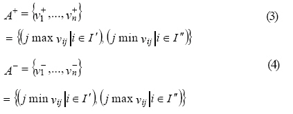
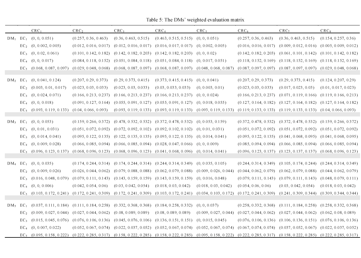
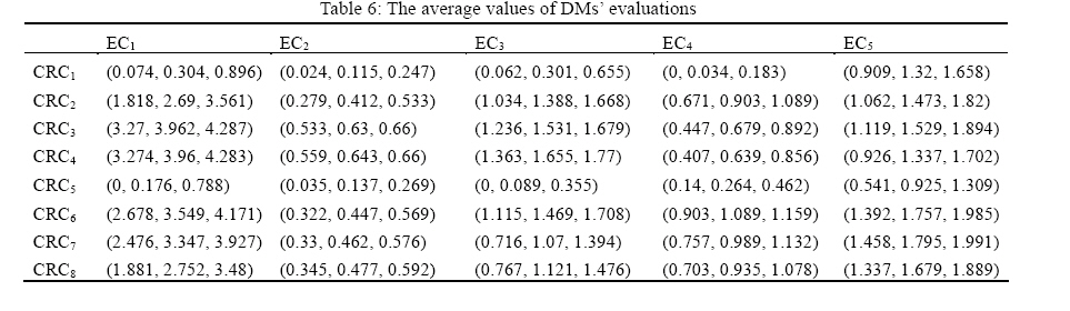
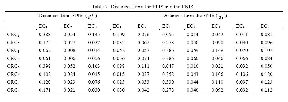
2. Calculate the weighted normalized decision matrix. The weighted normalized value vij is calculated as vij = wi rij , j = 1,..., J ; i = 1,..., n, (2) where wi is the weight of the ith attribute or criterion and Σn i =1wi =1. 3. Determine the ideal and negative-ideal solutions.
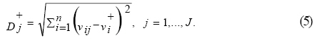
where I ' is associated with benefit criteria, and I " is associated with cost criteria. 4. Calculate the separation measures using the n-dimensional Euclidean distance. The separation of each alternative from the ideal solution is given as
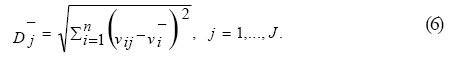
Similarly, the separation from the negative-ideal solution is given as
5. Calculate the relative closeness to the ideal solution. The relative closeness of alternative aj with respect to A+ is defined as
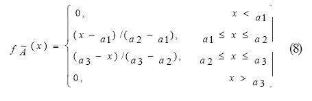
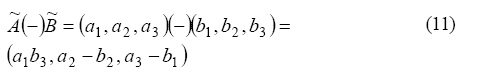
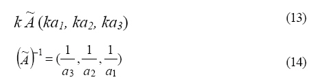
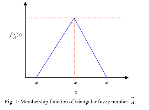
6. Rank the preference order Fuzzy sets Some definitions of fuzzy sets related with this study are given as following. Definition 1. A fuzzy set à in a universe of discourse X is characterized by membership function μà , which associates with each element x in X a real number in the interval (0, 1). The function à (X) is termed the grade of membership of x in (Chen, 2001). Definition 2. A triangular fuzzy number can be defined as a triplet (a1, a2, a3); the membership function of the fuzzy number is defined as in Figure 1. (Wang and Chang, 2007):
Let à and
Definition 3: The distance between triangular
fuzzy numbers à and
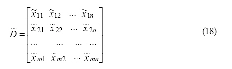
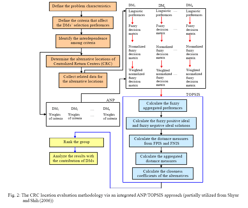
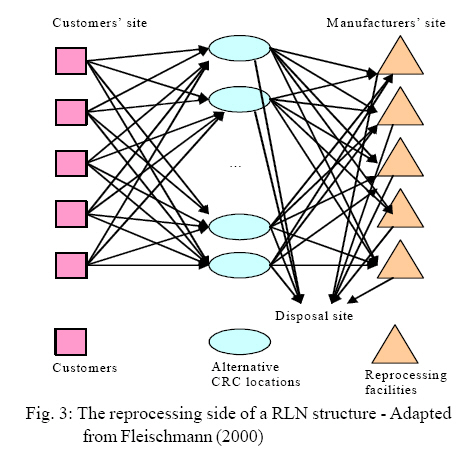
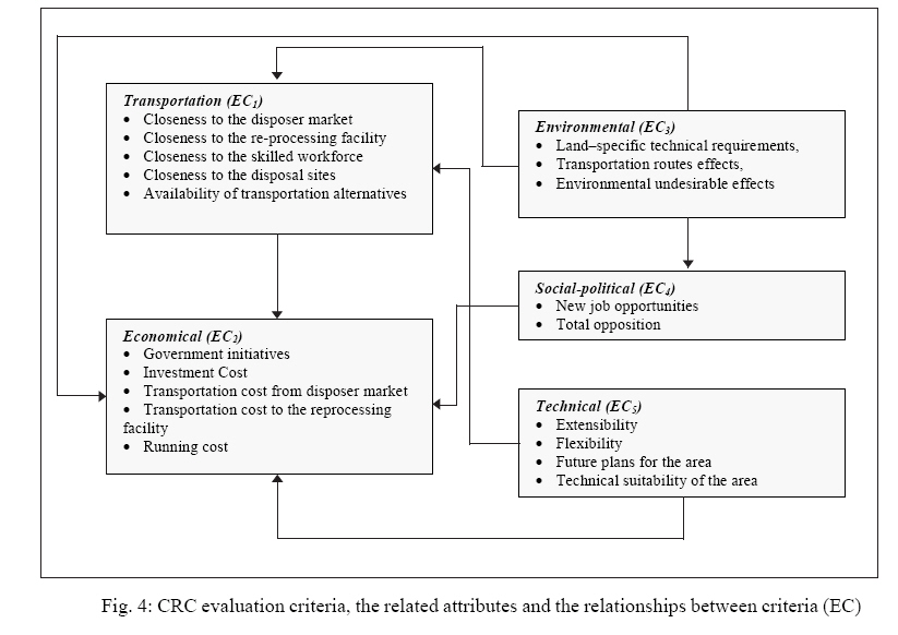
Definition 4. A linguistic variable is a variable whose values are linguistic terms (Chen, 2001). The concept of linguistic variable is very useful in dealing with situations which are too complex or too ill-defined to be reasonably described in conventional quantitative expressions. These linguistic variables can also be represented by fuzzy numbers (Chen, 2001). RESULTS AND DISCUSSION Proposed CRC location evaluation methodology: Integrated ANP-Fuzzy TOPSIS approach In this paper, a methodology that integrates the ANP and fuzzy TOPSIS techniques is utilized. The idea of the integration of ANP and TOPSIS techniques was first proposed by Shyur and Shih (2006) and Shyur (2006). Shyur and Shih (2006) presented the integrated approach for a strategic vendor selection problem. They first used ANP to obtain the relative weights of the criteria but not the entire evaluation process, reducing the large number of pair-wise comparisons required. They then used the modified TOPSIS function, which exploits a newly defined weighted Euclidean distance and aims to rank competing products in terms of their overall performance with multiple criteria. Shyur (2006) also used a very similar approach to a different problem named the commercial-off-the-self (COTS) evaluation and selection problem. Inspired by these two papers, this paper utilizes an integrated ANP and TOPSIS methodology for the centralized return center (CRC) location evaluation problem of a reverse logistics network (RLN) design problem. However, the specific problem requires fuzzy numbers to be used due to the vagueness of the problem. The general flow of the methodology is shown in Fig. 2. At the ANP stage of the methodology, the first step is to determine the weights of the criteria. Each decision maker (DM) is asked to pair-wise evaluate all proposed criteria without assuming interdependence between criteria (Shyur and Shih, 2006). The pair-wise comparisons are scaled with Saaty's 1-9 scale (Saaty, 1980). In this scale, 1 implies indifference, and 9 implies the total preference of one criterion over another. Once the pair-wise comparisons are completed, the local priority vector w1 is computed as the unique solution of Aw1 = λ max w1 (16) where λmax is the largest eigenvalue of pair-wise comparison matrix A. All obtained vectors are further normalized to represent the local priority vector w2 (Shyur and Shih, 2006). In the next stage of ANP, the effects of interdependence between the evaluation criteria are investigated. The DMs examine the impact of all criteria by using pair-wise comparisons. Various pair-wise comparison matrices are constructed for each of the criteria. These pair-wise comparison matrices are needed to identify the relative impacts of criteria-interdependent relationships. The normalized principle eigenvectors for these matrices are calculated and shown as column components in the interdependence weight matrix of criterion B, where zeros are assigned to the eigenvector weights of the criteria for which a given criterion is given (Shyur, 2006). The final step of the ANP approach is to integrate the interdependence priorities with the priority vectors of the criteria. This integration is prepared as follows (Shyur, 2006): wc= Bw2T (17) Following the ANP processes, the linguistic preferences of the DMs are queried. Then Chen's (2001) linguistic variables for the ratings are used which are: Very poor (VP) -(0,0,1), Poor (P) - (0,1,3), Medium poor (MP) - (1,3,5), Fair (F) - (3,5,7), Medium good (MG) (7,9,10), Good (G) (7,9,10) and Very good (VG) (9, 10, 10). Then the decision matrices for each DM are constructed. Let A1, A2, …, Am be possible alternatives and C1, C2, …, Cn be criteria with which alternative performances are measured. A fuzzy multi-criteria decision-making method can be concisely expressed in matrix format as
where Then the fuzzy decision matrix is normalized
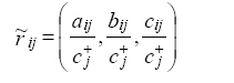
to eliminate anomalies with different measurement
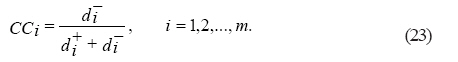
units. If where
Cj + = max cij The normalization method is needed to preserve the property that the ranges of normalized triangular fuzzy members belong to (0, 1) (Chen, 2000). At the next step, the weight of the criteria calculated via ANP is utilized, and the weighted normalized fuzzy decision matrices are calculated as
where wj represents the importance weight of criterion Cj. The next step consists of the stages of the fuzzy TOPSIS method. The elements of the weighted fuzzy decision matrix are normalized positive fuzzy numbers, and their ranges belong to the closed interval [0, 1] (Chen, 2000). Then, the fuzzy positive ideal solution (FPIS, A+) and the fuzzy negative ideal solution (FNIS, A-) can be defined as (Chen, 2000).
Then, the distance of each alternative A+ and A- can be calculated as (Chen, 2000):
where d (.,.) is the distance measurement between two fuzzy numbers. Then, the closeness coefficients are determined in order to rank the order of the alternatives. The closeness coefficient of each alternative is calculated as (Wang and Chang, 2007):
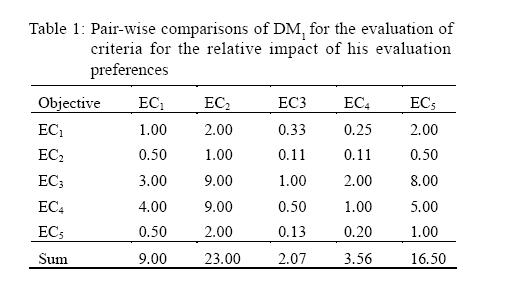
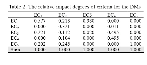
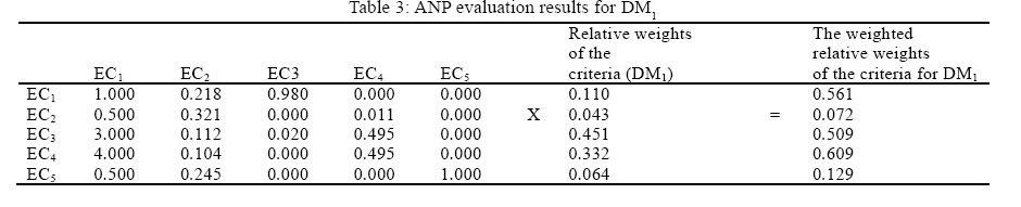
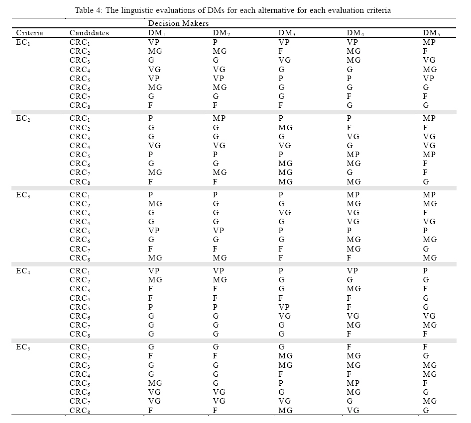
If values of CCi are close to "1", this indicates that the alternative is close to the FPIS. If values of CCi are close to "0", this indicates that the alternative is close to the FNIS. The application of the methodology and an illustrative example In this study, we are specifically interested in the evaluation of CRC location alternatives in a RLN structure. The general structure of the reprocessing side of a RLN is shown in Fig. 3. The customers' site of the market sends used products, labeled product A, to the appropriate CRC. In the CRC, the products are sorted, processed and shipped to their next destination, an appropriate re-processing facility or the disposal site. In the re-processing facility, the used products are re-processed, and waste parts are sent to a disposal site. In our illustrative example, eighth potential CRC location alternatives are shown: CRC1, CRC2, CRC3, CRC4, CRC5, CRC6, CRC7, and CRC8. The next step of the methodology is the criteria determination phase. The criteria for evaluating CRC location alternatives, related attributes and relationships between them are determined according to the related literature (especially Tuzkaya et al., in press), Vasiloglou (2004), Karagianniadis and Moussiopoulos (1998), Mahler and De Lima (2003), and Al-Jarrah and Abu-Qdais (2006)), and the DMs of the field such as municipal, environmental organization, disposer site and manufacturer site authorities (Fig. 4). In the first stage, the evaluation criteria are weighted for each DM using ANP. Here, five DMs contribute to the CRCs' evaluation: DM1 is from an environmental organizations' site, DM2 is from a municipal management's site, DM3 is from the consumers' site, DM4 is from the manufacturers' site and DM5 is from the CRC management's site. First of all, the DMs are asked to pair-wise evaluate the evaluation criteria for the relative impact of their evaluation preferences. Here, the DM1's pair-wise comparisons are given in Table 1. Then Table 1 is normalized via the column normalization technique, and the average values of the elements of the each row are taken. The relative weights of the criteria for DM1 are calculated as: 0.11, 0.043, 0.451, 0.332 and 0.064. In the next stage, the DMs are asked to evaluate the relative impacts of the criteria with respect to each other. In this stage DMs are grouped together and a compromise evaluation is handled (Table 2). Then, the relative impact degrees (Table 2) are weighted for each DM according to their preferences for the evaluation criteria (Eq.17). This step is illustrated in Table 3 for DM1, and the final evaluation results of the DM1 for EC1, EC2, EC3, EC4 and EC 5 is (0.515, 0.017, 0.203, 0.169, 0.097), DM2 for EC1, EC2, EC3, EC4 and EC 5 is (0.415, 0.033, 0.237, 0.182, 0.133), DM3 for EC1, EC2, EC3, EC4 and EC 5 is (0.532, 0.102, 0.135, 0.094, 0.137), DM4 for EC1, EC2, EC3, EC4 and EC 5 is (0.349, 0.088, 0.159, 0.060, 0.344) and DM5 for EC1, EC2, EC3, EC4 and EC 5 is (0.368, 0.089, 0.151, 0.074, 0.317). At the next stage, the evaluations of the DMs for each alternative and for each criterion are asked linguistically (Table 4). The preferences in Table 4 are converted to fuzzy numbers based on the Chen's (2001) scale. Here, triangular fuzzy numbers are preferred because for their ease of use. Then the fuzzy evaluations matrix is normalized using Eq. 19. At the next stage, the normalized fuzzy decision matrix is weighted according to the DMs' evaluations using Eq. 20. The results are shown in Table 5. At the next stage, the DMs' preferences are aggregated. Here, the DMs are assumed to have equal importance for the decision making process, hence the average values are calculated for the aggregation process (Table 6). Following this stage, FPIS and FNIS values are found according to Eq. 21. The FNIS and FPIS values of EC1 are (4.287, 4.287, 4.287), (0, 0, 0), respectively. The FNIS and FPIS values of EC2 are (0.66, 0.66, 0.66), (0.024, 0.024, 0.024), respectively. The FNIS and FPIS values of EC3 are (1.77, 1.77, 1.77), (0, 0, 0), respectively. The FNIS and FPIS values of EC4 are (1.159, 1.159, 1.159), (0, 0, 0), respectively. The FNIS and FPIS values of EC4 are (1.991, 1.991, 1.991), (0.541, 0.541, 0.541), respectively. Then, the distances from the FPIS and FNIS are calculated using Eq. 22 (Table 7). Finally, the total distance from the positive ideal solution, the total distance from the negative ideal solution and the closeness coefficients are calculated using Eq. 23 and closeness coefficients for CRCs (CCi) are calculated as (0.208, 0.644, 0.783, 0.724, 0.169, 0.789, 0.718, 0.678). Finally, the DMs are asked to negotiate the results, and the final results are found. According to the CCi values, the closest alternative to the FPIS is CRC6; also CRC3 and CRC7 have very close CCi values to CRC6. The closest alternative to the FNIS is CRC1. CONCLUSION This paper presents an integrated ANP-fuzzy TOPSIS approach for the CRC location evaluation problem of a RL network. In the literature, the RL network design problem has been investigated in various studies; however, the evaluation of CRC locations has not yet been investigated. This paper provides an evaluation tool for CRC locations in RLN design problems. The ANP approach is preferred to the AHP approach, because it provides the opportunity to evaluate interdependence between criteria. Due to the need for a large quantity of pair-wise comparisons, only the criteria-weighting side of the methodology is utilized from ANP. The remaining side uses TOPSIS in a fuzzy environment for the imprecise character of the CRC location evaluation problem. The fuzzy TOPSIS approach allows us to evaluate qualitative criteria in a flexible and systematic manner. In the future studies, the proposed tool may be integrated in RLN design problems. Hence, the assignment of customers to CRCs and CRCs to facilities can be made in a more systematic way. In such a study, the integration of meta-heuristics - such as genetic algorithms, simulated annealing, Tabu search, etc. - and the proposed methodology may be utilized. ACKNOWLEDGMENTS One of the authors, Gülfem Tuzkaya, is partially supported by the TUBITAK-Turkish Scientific and Technologic Research Association and wish to thank its financial support. REFERENCES
© IRSEN, CEERS, IAU The following images related to this document are available:Photo images[st08039t1.jpg] [st08039t3.jpg] [st08039t6.jpg] [st08039f3.jpg] [st08039t5.jpg] [st08039t2.jpg] [st08039t4.jpg] [st08039t7.jpg] [st08039f1.jpg] [st08039f4.jpg] [st08039f2.jpg] |
| |||||||||
