 |
| About Bioline | All Journals | Testimonials | Membership | News |
|
||||||
|
||||||
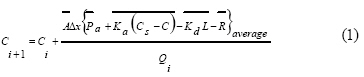
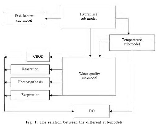
International Journal of Enviornmental Science and Technology, Vol. 6, No. 2, Spring, 2009, pp. 315-324 Impact of control structures on assimilative capacity of rivers and fish habitat *E. H. Imam; S. A. El Baradei Construction Engineering Department, American University, Cairo, Egypt Code Number: st09035 ABSTRACT This research studies the impact of water level control structures on self-assimilative capacity of rivers and on fish habitat. Constructing a water level control structure in a river reach will alter its hydraulics as well as its water quality, thermal regime and fish habitat. A mathematical model is developed to simulate river hydraulics, water quality, temperature and fish habitat. Diurnal dissolved oxygen concentrations are investigated to show their impact on fish. A case of a Nile River reach was studied to investigate the impact of the existence of the Esna barrage on the water quality and fish in its upstream reach. The barrage has negative impacts on the upstream self-assimilative capacity of the rivers. The waste load that the river could absorb was only 54 % (at low flow) and 78 % (at high flow) of the entire load if no barrage was present. Including in the simulation of the effects of photosynthesis and respiration, the above mentioned percentages were raised to 54 % and 91 %, respectively. Although water level control structures have negative impacts on the upstream self-assimilative capacity of the rivers, they have positive effect on downstream dissolved oxygen concentrations due to reaeration that happens across them. Downstream dissolved oxygen concentration increased by 6 % from its upstream concentration value. The barrage has a positive effect on fish habitat in the upstream section. The weighted usable area of Tilapia fish is doubled in case of barrage existence. The barrage causes a slight decrease in water temperature that reaches an average of 0.13 degree in the month of June. Keywords: Self-assimilative capacity, hydraulic structure, mathematical modeling, dissolved oxygen concentrations, photosynthesis and respiration, thermal regime and water temperature INTRODUCTION Control structures such as weirs and barrages constructed on a river will change the hydraulic regime of that river (Moffat et al., 1990) by increasing water depths and reducing velocities in the zones of developed backwater curves. This modified hydraulic regime impacts water quality due to changes in the transport and decay processes of pollutants along the rivers. Thus, the pollutant load will have a different impact on water quality after construction of the control structures as compared to the preconstruction stage. The modified hydraulic regime also impacts the thermal regime and fish habitat in the river. Although the construction of dams across rivers usually entails in-depth socio-economic and environmental impact studies, water level control structures are usually governed by their economic feasibility with limited attention to their in-stream environmental impacts. McCully (2001) studied the economic impacts of dams based on detailed investigation of economic and politic aspects of large dams. Numerous researchers have investigated the effects of hydraulic structures, which creation of impoundments similar to dams behind them, on water quality (Goldsmith and Hildyard, 1986) studies the environmental effects of large dams. Fewer studies have investigated the effect of water level control structures such as barrages and weirs on water quality and ecosystem health. Eid (1992) is among the rare researchers who investigated the impact of barrages on both water quality and fish habitat in rivers. However, that study used a simplified prismatic river section and considered only atmospheric reaeration and ignored photosynthesis. Eid studied the impact of barrages on fish habitat, but not the actual fish assemblage. Many studies such as (Barbie and Gandara, 1999; Idaho, 2004; Jacobs, 1994; Neumann, 2003; Shanahan, 1984; Wright et al., 1999) have simulated water temperatures from air temperatures, but did not consider the effect of hydraulic structures on water thermal regime. Eid studied this impact but, the simulated water temperature was assumed to be consistent with a linear relation and the lag time between water and air temperature wasn't considered. This paper studies the impact of water level control structures on the self-assimilative capacity of rivers and assesses possible changes in the ecosystem and fish habitat. For this purpose, water quality indicators were developed in order to express this impact in a quantifiable manner. This study was carried out in 2005 on the Esna barrage, in Egypt. MATERIALS AND METHODS The impact of constructing a water level control structure across a river is numerically modeled. The model consists of two main sub-models; a hydraulic sub-model and a water quality sub-model as described in Fig. 1. The water quality sub-model consists of a dissolved oxygen simulator along with its components such as biological oxygen demand, reaeration, photosynthesis and respiration. Two additional sub-models were developed: The temperature sub-model and the fish habitat sub-model. Hydraulic sub-model The hydraulic sub-model simulates backwater curves, velocities and areas for a controlled river reach of any geometrical shape using the standard-step method (Chapra, 1997; Chou, 1988; French, 1985). Dissolved oxygen (DO) sub-model The DO sub-model simulates all available sources and sinks except nitrogenous biological oxygen demand (NBOD) and sediment oxygen demand (SOD). A mass-balance equation can be defined as follows:
Where,
Ci+1= DO concentration at section i+1 in
mg/L; Ci = DO concentration at section (i) in mg/L; = average area of sections i and i+1 in m2;
The sources and sinks of Eq. 1 are explained in the following paragraphs: In Eq. 1, all sources and sinks are taken to be the average of their concentrations between sections (i) and (i+1).
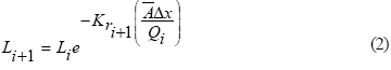
Where, Li+1= CBOD concentration at section i+1
in mg/L; Li = CBOD concentration at section i in
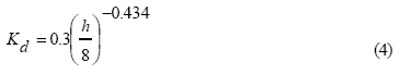
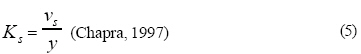
mg/L; Kr = Kd + Ks Where, Kd = decomposition rate of CBOD in the stream/day; Kd = settling rate of CBOD/day. There are more than one way to obtain Kd (McDonnell and Wright, 1979; Thomann and Mueller 1987). The following equation of Thomann is used in this study:
(Thomann, 1987);
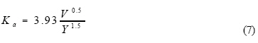
Where, y = average water depth in m; vs= settling velocity in m/day. The exchange of air at the surface of the water body makes use of the "two film theory", which assumes that a gaseous film is at the atmosphere side of the air-water interface and a liquid film is at the water side of the interface. For oxygen to transfer from the atmosphere to the water, a parcel of water must first travel from the bulk liquid to the interface. Oxygen can then diffuse to the water parcel, through the gaseous film and through the liquid film (Thomann and Mueller 1987): Reaeration = Ka(Cs -C) (6) Where, Ka = volumetric reaeration coefficient/day. To obtain Ka, O'Connor-Dobbins formula is used
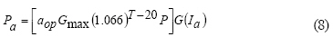
Where; V = average velocity; Y = average depth in m; Cs = saturation concentration of DO at certain section in mg/L; C = DO concentration at certain section in mg/L. The average of the reaeration equation is taken between two successive sections of the control volume. The essence of photosynthetic process centers about chlorophyll a -containing plants which utilize radiant energy from the sun, convert water and carbon dioxide into glucose and release oxygen. Thus, production of oxygen happens only during daylight hours. The variation of light and hence photosynthesis can be idealized by a half sinusoid function, from day to day (maximum value of photosynthesis happens at noon and minimum value happen at sunrise and sunset). Thus, swings in oxygen can be induced by diurnal light variations. Where, Pm= maximum rate in g/m3d; tr= time of sunrise in day; ts= time of sunset in day; f = fraction of day subject to sunlight (the photoperiod); Tp = daily period (1d, 24 h, etc. depending on the units of time) A method called "Estimation from observed chlorophyll levels" is used to estimate the value of the photosynthesis over the control volume. This method assumes that the phytoplankton is the principal source of oxygen. Actually phytoplankton are floating plants that dominate throughout deep rivers. On the other hand, in shallower streams, where light can reach the lower depths, bottom plants would tend to make up most of the plant biomass. These can include rooted and attached plants. This method requires a direct measurement of the concentration of phytoplankton as represented by chlorophyllin the water. Since photosynthesis is light dependent, the relationship between phytoplankton chlorophyll and photosynthetic production depends on solar radiation, depth and the extinction coefficient. This is described through the following equations (Thomann and Mueller 1987).
Where, Pa = daily average growth production (photosynthesis) in mg DO/L/day; aop = mg of DO/µg of chla means chlorophylla; P = phytoplankton chlorophyll in µg/L; Gmax = maximum growth rate of the phytoplankton at 20 °C /day; T = temperature (°C); G (Ia) = light attenuation factor over depth and one day (Unitless). Respiration is the process by which organisms take up oxygen and discharge carbon dioxide in order to satisfy their energy requirements. Eq. 9 simulates the effect of the respiration process. R = aop (0.1)(1.08)T-20p (9) Where, R= phytoplankton respiration in mgDO/L/day. In addition to the atmospheric reaeration that happens to the river, there is another reaeration process that takes place across control structures. This is because the control structure will enhance the formation of hydraulic jumps in the water and thus allows more air to enter into the stream. This process has a positive effect on the DO concentration at the downstream side of the structure, because an added source to the DO equation is created. This is calculated by Gameson's equation: (ADEM, 2001) r = 1 + 0.11(a )(b)(1 + 0.046(T ))h (10) Where, r = ratio of upstream DO deficit to downstream deficit; a = water quality factor; b = structure aeration coefficient; T = water temperature (°C); h = water level difference across the dam (ft). Temperature sub-model Water temperature is vital for fauna and flora of water and also for chemical and biological reactions in rivers. Water temperature depends on air temperature (Group work, 1997; Pilgrim et al., 1998; Song et al., 1973) on hydraulic parameters of rivers such as depth of water and geometry of river sections. Constructing a water level control structure alters the hydraulic regime of water and thus may alter its thermal regime (John, 1984). Heat transferred at the air-water interface is the major factor that induces variation in water temperature. Many studies have shown that air and water temperatures are correlated. This is because water temperature depends on meteorological conditions that are represented through the air. Response coefficients representing the rate of water temperature variation with respect to the air temperature variation were found to correlate well (Song and Chien, 1977). The U.S Geological Survey Department studied some rivers in Texas and concluded that large streams have a small diurnal temperature change (Barbie and Gandara, 1999). Water temperature and its change depend on the water depth. Stefan and Preud’homme, (1993) revealed that the time lag which exists between the air and water temperatures varies linearly with the depth of the river. Also, they studied water temperature simulation as a result of the lag time between the air and the water temperatures. This study was carried out on 11 streams in the central U.S. (Mississippi River basin) and a linear equation correlating seasonal water temperature to seasonal air temperature was formed. This equation took into account the lag time between air and water temperatures. From this study, it was concluded that measured water temperatures follow the air temperatures closely with some time lag. Diurnal simulation of water temperature using air temperature was done by expanding the equation of (Stefan Stefan and Preud’homme, 1993) to accommodate the diurnal water temperature changes. This is described via Eqs. 11-13. Eq. 11 shows that the water temperature calculated at time (t) is a function in the air temperature at the time (t) less than the lag time.
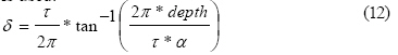
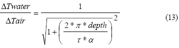
Where, the time (t) and the time lag (δ) are in units of days and temperatures are in °C. To calculate the lag time (d) the following equation is used:
Where, τ = cyclic period over which the study is done (here
24h); α = thermal diffusivity coefficient:
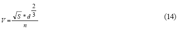
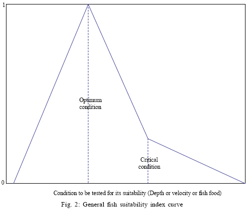
Fish habitat sub-model Fish is affected greatly by hydraulic parameters such as depth (Hepher, 1981) and velocity of water, which are affected by water level control structures. In this research, the Tilapia genus of fishes is studied, because it is the most widely spread fish in the Nile River, in Egypt. The general theory behind fish habitat modeling is based on the fact that aquatic species will react to changes in the hydraulic environment. These changes are simulated for each computational cell in a defined stream reach. The indication of the effect of the water level control structure on the fish habitat is expressed as the weighted usable area that fish will live in, which is estimated from suitability indices. A suitability index measures the conditions that are suitable for the fish to live under, has an upper bound "1", which reflects the optimum conditions for a certain kind of fish and a lower bound of "0" that represents the critical conditions for the fish (Fig. 2). There are suitability indices for hydraulic or physical conditions of fish habitat, including depth, velocity and food of the fish. Calculation of the 2-D velocity distribution across a section, as well as the average velocity of the section is carried out. This is done according to Eq. 14 (Habitat modeling, 2002):
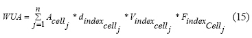
Where, V = velocity of computational cell in m/s; d = depth of computational cell in m; S = slope of the river bed in m/m and n = manning coefficient of cell. The velocity and depth of cell are taken as the average between their values at two successive vertical coordinates. The weighted usable area is weighted according to the load of each suitability index parameter and is given by:
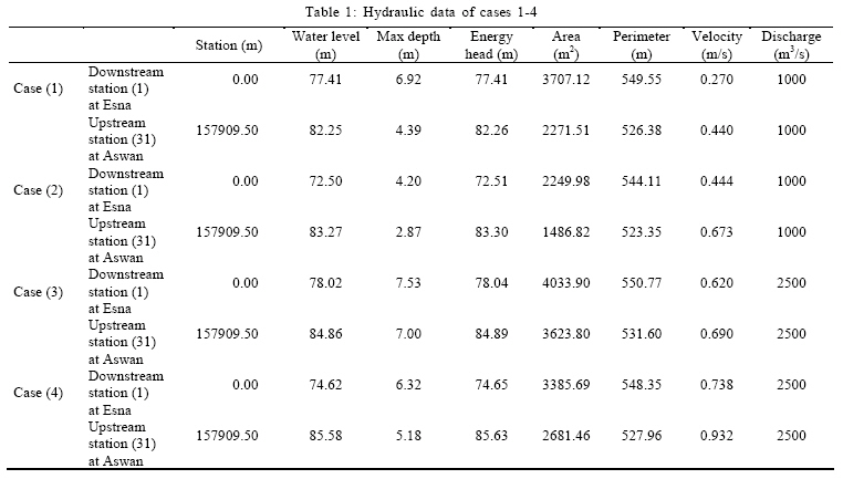
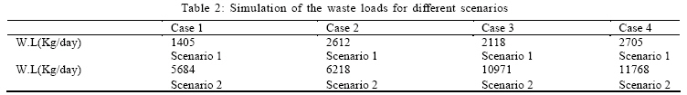
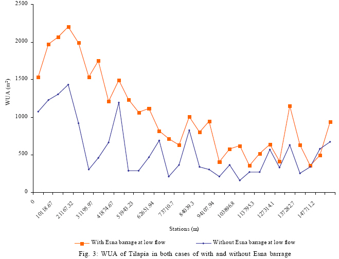
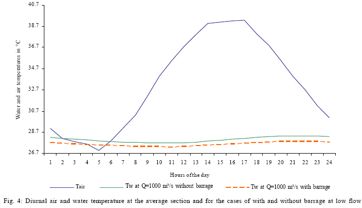
Where, F is the food of the fish. Assessment of the self-purification capacity and ecosystem The self-purification capacity of a river is the capacity of its water to accept different waste load concentrations without changing its original quality. To assess the impact of water level control structures on the self-assimilative capacity of rivers in a quantifiable manner, many indicators were developed. The effect of water level control structures on self-assimilative capacity of a river is assessed through introducing waste loads from point sources at different sections along that river. DO concentrations in the river is kept at a constant level of 5 mg/L. Waste loads are introduced to the stream from point sources at different sections along the river to be able to compare between the loading capacity of the river at different hydraulic cases. The effects of temperature and photosynthesis on diurnal DO variation are tested. Downstream DO concentration as a result of reaeration across the water level control structure is also calculated. This is important, because this reaeration increases DO levels at the downstream side of the structure. The presence of a water level control structure in a river or a waterway not only affects the water quality of that river, but it also affects the whole environment and ecosystem in the reach where it was constructed. Therefore, as indicators to this impact, the fish habitat and the thermal regime of the river are studied. Water temperature is important because it affects the biological and chemical processes in the water and thus, the CBOD and the DO concentrations. Existence of a water level control structure will alter water temperature in a controlled river reach. To study this effect, the diurnal change in water temperature is simulated for the four main hydraulic cases. Each kind of fish has its own physical condition requirements such as water velocity, depth, and the availability of food for the fish under which it can be best survived. Water level control structures in rivers alter their hydraulic regime and hence the physical factors that affect the fish population. This effect is assessed through calculating the WUA of fish for both cases of existence and non-existence of the structure. Case study of Nile River (Aswan-Esna reach) The case study investigates the effect of Esna barrage on the water hydraulic regime, as well as on water quality upstream of the barrage from Esna to Aswan. Hydraulic simulation of Aswan-Esna reach (upstream the barrage) The Esna-Aswan reach is 157.9 km long (Abdelbary, 1992). The peak discharge of the high dam is about 2500 m3/s (high flow conditions) and it occurs in July, whereas, the minimum discharge is about 1500 m3/s (low flow conditions) and occurs in January. Available river sections are every 5 km and interpolation was used to generate sections every 100 m in order to do hydraulic calculations via the standard step method in an accurate way. Manning coefficient is assumed to be constant (n=0.0287) throughout the simulated reach. The studied reach was simulated under four main hydraulic cases: Cases 1 and 2 study the existence and the non-existence of Esna barrage, respectively at low flow conditions; cases 3 and 4 study the existence and non-existence of barrage, respectively at high flow conditions. The results of the calculations and the water level profiles are summarized in Table 1 (El Baradei, 2005). Self-purification capacity and waste load at Aswan-Esna reach Two scenarios were simulated to compare between different cases of waste loadings (W. L). Scenario (1) uses the DO as a function of only CBOD and reaeration. Scenario (2) adds photosynthesis and respiration to the DO. Table 2 summarizes all the waste loading cases. (Imam and El Baradei, 2006). Diurnal dissolved oxygen DO concentration changes during the 24 h of the day because of change in water temperature and photosynthetic action of plants throughout the day. Minimum DO concentrations usually occur in the early morning while maximum concentrations occur in the early afternoon (Murphy, 1987). In the simulation, a section with average properties (hydraulics and water quality) was taken using simulated diurnal water temperature. The simulation compared the diurnal DO at cases of existence and non-existence of the barrage. In order to investigate the effect of the photosynthesis on the diurnal DO, a trial was done using only the CBOD and the reaeration in calculating the DO as opposed to another trial using the photosynthesis. The curve representing the diurnal DO in case of with the barrage was found to be slightly higher than that curve of the diurnal DO without the barrage. Hence, this is because the diurnal water temperatures in the presence of the barrage are less than those when no barrage is present; because with the barrage the depths are greater and DO fluctuations are less. In this case, water temperature is the parameter that has the greater effect on diurnal DO concentrations and it is known that the temperature is inversely proportionate with the DO concentration. Reaeration across the barrage (downstream DO concentrations) Gameson equation simulated DO concentrations downstream of the barrage. The calculations done under low flow conditions revealed an upstream DO concentration of 8.02 mg/L, an upstream DO deficit/downstream DO deficit of 3.90 and a downstream DO concentration of 8.49 mg/L. Simulation of the ecosystem at the Aswan-Esna reach- fish habitat The weighted usable area (WUA) of Tilapia fish was calculated in both cases of barrage existence and non-existence. Suitability indices of depth and velocity for Tilapia were constructed based on actual values. Food of Tilapia consists of the greatest part of phytoplankton which dwells in the first 1.5 m below water surface. Thus, the optimum depth for Tilapia is 1.5 m. The critical depth is 9 m. The optimum velocity is 0.3 m/s and the critical is 0.6 m/s. The suitability index for the availability of fish food is taken as unity. The WUA in case 1 is 31236.8 m2, whereas in case 2 it is 17061.93 m2. Fig. 3 compares between the WUA of cases 1 and 2 for the whole studied reach. The curve of case 1 is always higher than that of case 2. Simulation of the water temperature The effect of Esna barrage on the thermal regime of water was tested. The simulation of diurnal variation in water temperatures on a day in the month of June was done for one section that is representative for the whole reach. The water depth of this section is equal to the average of all water depths of all sections of the river reach. The simulation is done for the previously mentioned, four main hydraulic cases. It is observed that the sinusoidal diurnal water temperature curve follows the air temperature curve but with a lag time between water and air temperatures. This lag time increases with increased depth. Fig. 4 shows the diurnal air temperature curve, along with the diurnal water temperature curves at both cases 1 and 2. In case 1, the lag time between air and water temperatures is 5.842 h, whereas in case 2, it was 5.791 h. The curves show that in case 2, the diurnal water temperature is higher than that in case 1. Therefore, in case 2, the maximum water temperature during the whole day is 28.4 °C, whereas in case 1, it decreases to 27.8 °C. This indicates that the barrage causes a decrease in water temperature. During operating under high flow conditions, the diurnal water temperature further decreases. Thus, in case 4, the maximum water temperature during the whole day is 27.5 °C, whereas in case 3, it decreases to reach 27.3 °C (El Baradei, 2005). RESULTS AND DISCUSSION The drawn conclusions are general for any water level control structure, but the calculated percentages are of the Esna barrage case study categorized as follows:
REFERENCES
© IRSEN, CEERS, IAU The following images related to this document are available:Photo images[st09035f3.jpg] [st09035t1.jpg] [st09035f2.jpg] [st09035t2.jpg] [st09035f1.jpg] [st09035f4.jpg] |
| |||||||||
