International Journal of Environment Science and Technology Center for Environment and Energy Research and Studies (CEERS) ISSN: 1735-1472 EISSN: 1735-2630 Vol. 6, Num. 3, 2009, pp. 509-519

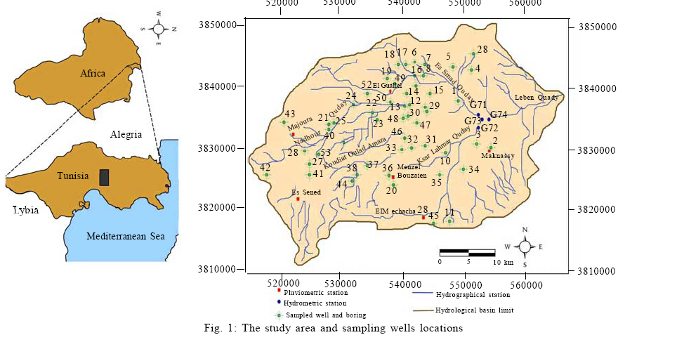
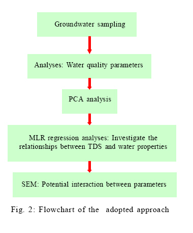
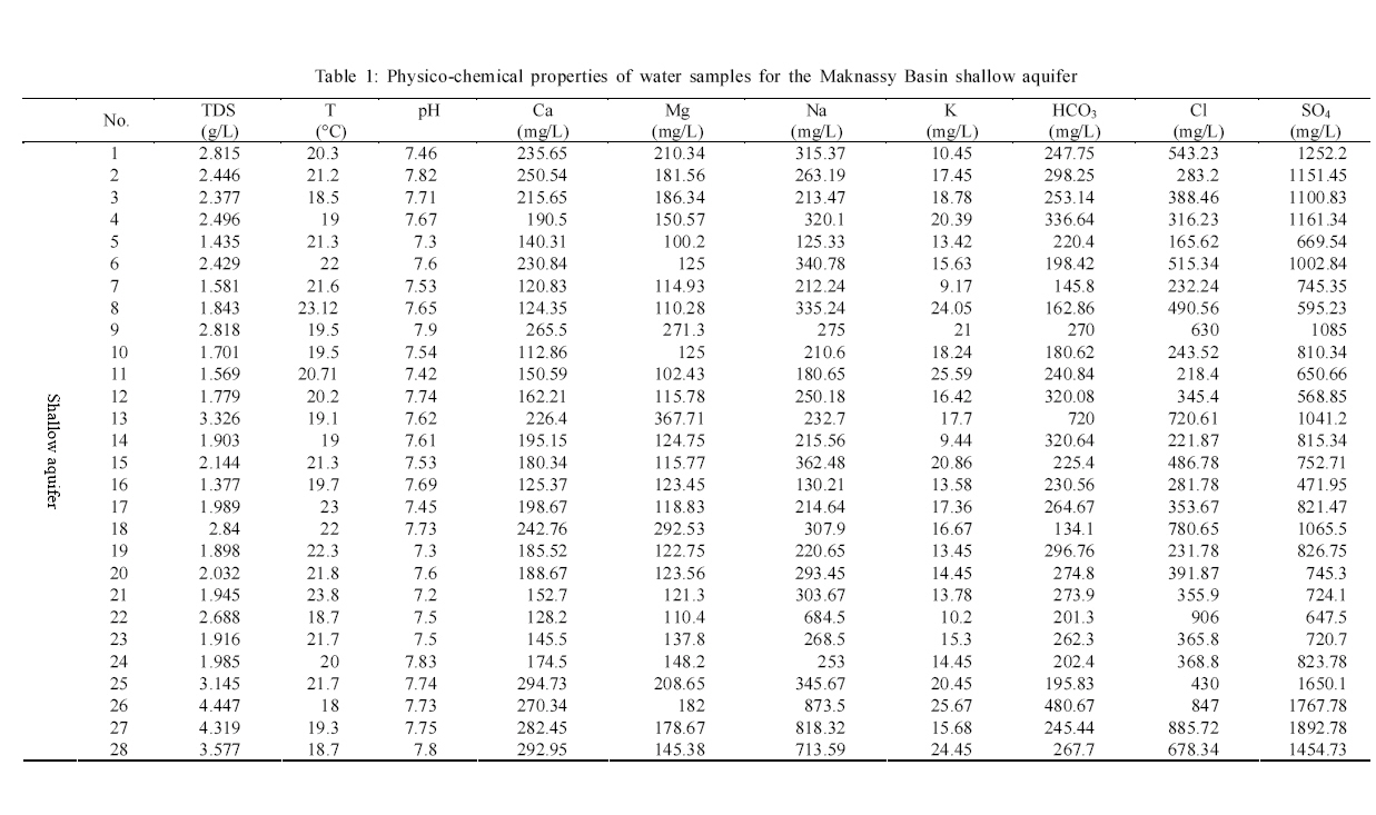
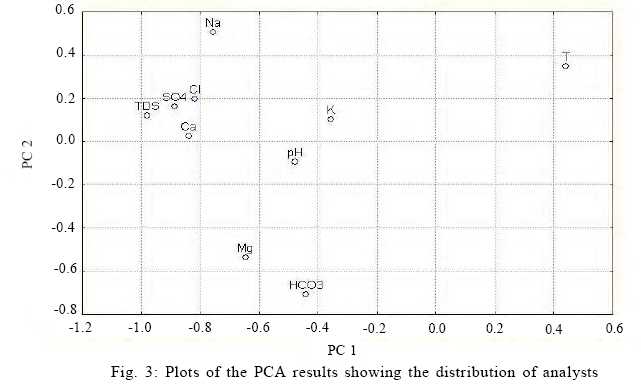
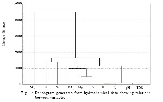
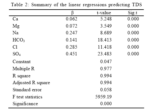
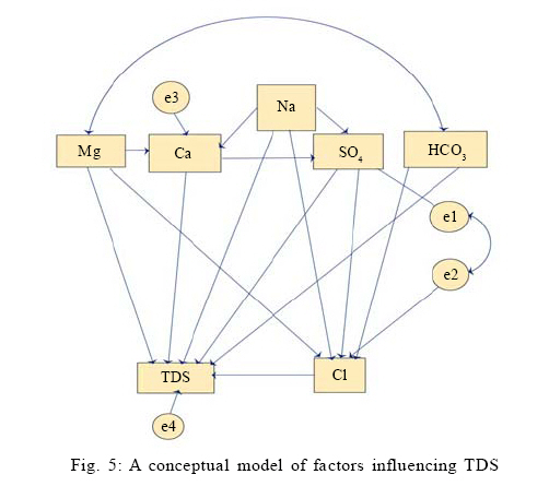
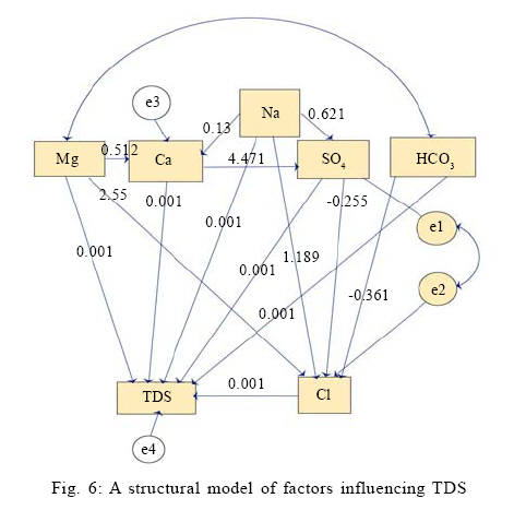
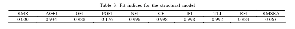
International Journal of Enviornmental Science and Technology, Vol. 6, No. 3, Summer, 2009, pp. 509-519

Evaluation of ground water quality using multiple linear regression and structural equation modeling

¹ *I. Chenini; ² S. Khmiri

¹ Minerals Resources and Environment Laboratory, Department of Geology, Faculty of Sciences of Tunis, 2092 Tunis El Manar, Tunisia
² U. R. Structural and applied geology, Department of Geology, Faculty of Sciences of Tunis, 2092 Tunis El Manar, Tunisia
*Corresponding Author Email: chenini_ismail@yahoo.frTel.: +216 97 282 335; Fax: +216 70 860 325

Received 2 January 2009; revised 18 April 2009; accepted 5 May 2009

Code Number: st09056

ABSTRACT

A methodology for characterizing ground water quality of watersheds using hydrochemical data that mingle multiple linear regression and structural equation modeling is presented. The aim of this work is to analyze hydrochemical data in order to explore the compositional of phreatic aquifer groundwater samples and the origin of water mineralization, using mathematical method and modeling, in Maknassy Basin, central Tunisia). Principal component analysis is used to determine the sources of variation between parameters. These components show that the variations within the dataset are related to variation in sulfuric acid and bicarbonate, sodium and cloride, calcium and magnesium which are derived from water-rock interaction. Thus, an equation is explored for the sampled ground water. Using Amos software, the structural equation modeling allows, to test in simultaneous analysis the entire system of variables (sodium, magnesium, sulfat, bicarbonate, cloride, calcium), in order to determine the extent to which it is consistent with the data. For this purpose, it should investigate simultaneously the interactions between the different components of ground water and their relationship with total dissolved solids. The integrated result provides a method to characterize ground water quality using statistical analyses and modeling of hydrochemical data in Maknassy basin to explain the ground water chemistry origin.

Keywords: Ground water quality; Hydrochemical; Mathematical method; Water-rock interaction

Introduction

Water quality concept has been evaluated in the last years owing to greater understanding of water mineralization process and greater concern about its origin (Shane and Jerzy, 2003). Water quality shows water-rock interaction and indicates residence time and recharge zone confirmation (Cronin et al., 2005). Thus, water quality indicators must reflect mineralization process, integrate reservoir properties and be sensitive to ground water recharge rate and flow direction (Andre et al., 2005). The concept of ground water quality seems to be clear, but the way of how to study and evaluate it still remains tricky. The chemical composition of ground water is controlled by many factors that include the composition of precipitation, mineralogy of the watershed and aquifers, climate and topography. These factors can combine to create diverse water types that change in composition spatially and temporally. The use of major ions as natural tracers has become a common method to delineate flow paths in aquifers (Back, 1966). Generally, the approach is to divide the samples into hydrochemical facies, that is groups of samples with similar chemical characteristics that can then be correlated with location. The observed spatial variability can provide insight into aquifer heterogeneity and connectivity, as well as the physical and chemical processes controlling water chemistry. In recent decades, multivariate statistical methods have been employed to extract significant information from hydrochemical datasets in compound systems. These techniques can help resolve hydrological factors such as aquifer boundaries, ground water flow paths, or hydrochemical components (Liedholz and Schafmeister, 1998; Locsey and Cox, 2003; Seyhan et al., 1985; Suk and Lee, 1999; Usunoff and Guzman-Guzman, 1989) identify geochemical controls on composition (Adams et al., 2001; Alberto et al., 2001; Lopez-Chicano et al., 2001; Reeve et al., 1996). Different techniques have been used in attempt to evaluate water quality, essentially based on chemical ions correlation (Piper and sholler diagramm) and some ions rapports to predict the origin of the mineralization (Bennetts et al., 2006; Pulido-Leboeuf et al., 2003). Chemometric analyses were used to differentiate the water samples on the basis of their composition and origin (Singh et al., 2005). The present study attempts to establish a mathematical water quality model. Since the data obtained in this study had multivariate nature and several of the variables were correlated, Principal component analysis (PCA) analysis methods were used for the interpretation of the data. Multiple linear regression (MLR), based on chemical ground water properties in phreatic aquifer level in Maknassy basin, is given as an accurate tool to evaluate ground water quality, since it generates a minimum data set of indicators (Doran and Parkin, 1996). Then, all the variables would be included simultaneously into single model in order to test the potential interactions between the independents variables using the structural equation modeling (SEM). Therefore, the results of ground water quality data analyses in a sequential fashion have been fully integrated to better constrain the interpretation and include the statistical modeling in the process. Sampling and ground water analysis were done in Minerals Resources and Environement Laboratory, in October 2006.

Materials and methods

The study site covers an area of about 1250 km² located in southern central Atlas of Tunisia. In this geographic area, climate is arid Mediterranean type. The study basin has a three tiers aquifer system. The shallow aquifer extending to varying depths of 30-150 m; the deep aquifer made up by two fractured limestone levels extending to depth between 180 and 250 m and the upper level of deep aquifer forms the main source of water supply in the studied area. The altitude of water table in the region varies from 180 to 320 m and movement of ground water is from east to west and from borders to center basin (Chenini et al., 2008). The sampling network and strategy were collected in equilibrium state of aquifer, which reasonably represent the ground water quality in the study region. A total of 28 water samples were collected in the months of October-November 2005 (Fig. 1). All the samples, collected in tight capped high quality polyethylene bottles, were immediately transported to the laboratory under low temperature conditions in ice-box and stored in the laboratory at 4 °C until processed analyses. All analyses were completed within a week time in laboratory. The measured variables included the characteristic water quality parameters. Temperature was measured on the site using mercury thermometer. All other parameters were determined in laboratory following the standard protocols (Apha, 1985). The ground water samples were analyzed for parameters which include pH, electrical conductivity (EC), total dissolved solids (TDS), bicarbonates (HCO₃ ^-), chloride (Cl^-), sulfate (SO₄²⁺), sodium (Na⁺), potassium (K⁺), calcium (Ca²⁺) and magnesium (Mg²⁺). Electrical conductivity was measured at 25 °C with a conductivity meter. pH was measured using a pH-meter. Major anions were analyzed using modular ion chromatograph. Among the major cations, sodium, potassium, calcium and magnesium were analyzed by flame photometer. TDS were determined grametrically. The analytical data quality was ensured through careful standardization; the ionic charge balance of each sample was within ± 5 %. The ground water ionic strength is dominated by major cations and anions. Hydrochemistry of the phreatic aquifer of Maknassy Basin was summarized through the statistical analysis and mathematical modeling of ground water properties. Before establishing the statistical models, the detection of outliers and the elucidation of trends, similarities and dissimilarities among chemical properties of sampled water were carried out according to PCA method (Jolliffe, 2002; Muller et al., 2008). As a multivariate data analytic technique, PCA reduces a large number of variables to a small number of variables, without sacrificing too much of the information (Qian et al., 1994). More concisely, PCA combines two or more correlated variables into one variable. This approach has been used to extract related variables and infer the processes that control water chemistry (Helena et al., 2000; Hidalgo and Cruz-Sanjulian, 2001). PCA method was performed using STATISTICA 6.0 statistical program. The general purpose of multiple linear regressions is to quantify the relationship between several independent or predictor variables and a dependant variable. This method is successfully used by different authors to establish statistical model (Ghasemi and Saaidpour, 2007).

MLR method provides equation linking a dependant variable Vd ([Na], [Mg], [SO₄], [HCO₃], [Cl], [Ca]) to the independent variable Vi using the following form:

Vd = β₀ + β₁ V_i1 + ... + β_n V_in

When the intercept β₀ and the regression coefficients of descriptors (β_i) are determined by least square method (Green and Carroll, 1996). Vi descriptors are used to describe water quality and cation dependence. (n) is the number of water samples. The reduction in the number of descriptors (variables) is included in the study to minimize the information overlap in variables. The best equation is selected while being based on the highest multiple correlation coefficients (R), lowest standard deviation (SD) and F-ratio value. Relationships between variables were established using the forward stepwise regression method (Bernstein, 1988). The MLR modeling method was performed by the SPSS statistical program. Structural equation modeling is a statistical method that takes a confirmatory fashion to the analysis of a structural theory bearing on some phenomena (Kline, 2005). Typically this theory represents “causal” processes that generate observations on multiple variables (Bentler, 1988). The SEM conveys that the causal processes under study are represented by a series of structural equations and that these relations can be modeled. The model can then be tested statistically in a simultaneous analysis of the entire system of variables to determine to which it is consistent with the data. Several aspects of SEM set are apart from the older generation of multivariate procedure (Fronell, 1982). First, it takes a confirmatory, rather than an exploratory, approach to the data analysis. Furthermore, SEM lends itself well to the analysis of data for inferential purpose. In the other hand, must other multivariate procedures are essentially descriptive by nature, so that hypothesis testing is difficult. Second, although traditional multivariate procedures are incapable of either assessing of correcting measurement error. SEM provides explicit estimates of these error variance parameters (Byrne, 2001). The data were input to Amos 7.0 (Arbuckle, 2006) for SEM analysis. The flowchart of Fig. 2 summarizes the steps of the study.

RESULTS AND DISCUSSION

PCA was applied to the combined ground water data set of the shallow aquifer (Table 1) to examine relations between water properties analyzed and to identify the factors that influence the concentration of each one. According to PCA, the three significant PCs are cumulatively accounted for 70 % of the total data variance. Most of the variance is contained in PC1 (48.4 %), which is associated with the variables [Na], [Cl], [Ca], [SO₄] and TDS. PC2 explains 12.6 % of the variance and is mainly related to [Mg] and [HCO₃]. The variables pH, [K] and T contribute most strongly to the third component (PC3) that explains 10.2 % of the total variance. PC1 contains hydrochemical variable originating from weathering process and reservoir formation dissolution, whereas PC2 and PC3 are related to bicarbonates and physical properties. Fig. 3 shows the projection of the first two PC scores in a scatter plot. The distribution suggests a more continuous variation of properties of the samples. The application of PCA reveals that the classification of ground water sampled was achieved according to their chemical and physical properties. The analysts (chemical properties) were classified and presented in a dendogram (Fig. 4). It confirms the PCA classification, but TDS is grouped with pH, [K] and T. [SO₄] is important in water samples that's why it can be classified as an own class of water properties. 7 analysts were randomly selected to constitute the training set for the construction of statistical models. Regression analysis (SPSS 14.0) was conducted to investigate the relationships between TDS and water properties. The [Na], [K], [Mg], [SO₄], [HCO₃], [Cl], [Ca] were considered as independent variables and TDS as a dependent variable. The best model was derived by the application of MLR method. After obtaining various equations with ground water samples from the phreatic qauifer levels. An analysis of residuals was developed and R² values were studied. Among all candidate equations, the equation where this ratio was closer to 1 were selected. The descriptors and the regression coefficient of this model are presented in Table 2. As can be seen in the case of all the MLR regression analyses, the water properties measures are statistically significant in estimating TDS (P < 0.00). The multiple R coefficient indicates that the correlation between water properties and TDS is moderate (the multiple R > 0.99). According to R square statistic, 99 % for the total variance for the estimation of TDS is explained by the MLR model. The model was also checked to see if it was prone to any multicollinearity effect. The Variance Inflation Factor (VIF) value obtained was close to one and thus, there was no evidence of multicollinearity (Hair and Anderson, 1998). In terms of the relative importance of the estimation of a dependent variable, it can squabble that the [SO₄] makes the largest contribution across the model. An examination of t-values also reveals an identical descending order of the factors that contribute to the estimation of TDS in Maknassy basin phreatic aquifer water (Bring, 1994). The positive sign of the beta coefficients and t-values pertaining to these variables indicates that there is a positive relationship between TDS and elements of ground water properties ([Na], [Mg], [SO₄], [HCO₃], [Cl], [Ca]). The selected equation for shallow aquifer ground water in Maknassy basin is:

TDS = 0.047 + 0.072 Mg + 0.062 Ca + 0.247 Na + 0.285 Cl + 0.141 HCO₃ + 0.451 SO₄ + ε (2)

Where, ε is the error of estimation in the statistical regression model.

The second step of this study includes simultaneously all the variables in a conceptual model in order to test the potential interaction between them. The structural equation modeling was used to achieve the goal. A generalized conceptual model was developed which is illustrated in Fig. 5. This model hypothesizes the potential interactions between the independents variables (Na, Mg, SO₄, HCO₃, Cl, Ca) and their contribution on the dependant variable (TDS). e1, e2, e3 and e4 are added to the statistical model in order to reduce the error estimation of path value (relation) between variables. TDS in ground water sampled is constrained by [SO₄], [HCO₃] and [Cl] result of water-rock interaction. Thus, the sulphated facies ground water could be remaining to the dissolution and/or leaching of the abundant gypsum in geological formations and soil in Maknassy basin.

Fig. 5 depicts the causal relationship among exogenous and endogenous variables. An exogenous variable's causes lie outside the model. In these causes, [Na], [Mg] and [HCO₃] are the exogenous variables in the structural model. In contrast to exogenous variables, the postulated causes of endogenous variables are included in the model. In the current model (Fig. 6), TDS, [Ca], [SO₄] and [Cl] are all endogenous variables. All factors loadings that were tested had t-values greater than 1.96 and all of the path coefficients were significant. The goodness of fit indices for the structural model that are shown in Table 3 indicated the model has a good fit of the data. The root mean square (RMR) residual represents the average value across all standardized residuals and ranges from 0 to 1; in a well-fitting model this value will be smaller than 0.05. Turning to Table 3, it can be seen that the RMR value for this model is 0.000. It is concluded that the model fit the data well. The adjusted goodness of fit index (AGFI) differs from the goodness of fit index (GFI) only in the fact that it adjusts for the number of degree of freedom in the specified model. They address the issue of parsimony by incorporating a penalty for the inclusion of additional parameters. The GFI and AGFI can be classified as absolute index of fit (Bentler, 1990). Although, both indices range from 0 to 1, with values close to 1 being indicative of good fit. For Joreskog and Sorbom (1993) this two indices is impossible for them to be negative. Fan et al. (1999) further cautioned that GFI and AGFI values can be overly influenced by sample size. Based on GFI and AGFI values reported in Table 3 (0.988 and 0.934, respectively), it can be, once again, concluded that this model fits the sample data fairly well. Parsimony goodness fit index (PGFI), was introduced to address the issue of parsimony in SEM. The PGFI takes in to account the complexity (i.e., number of estimated parameters) of the hypothesized model in the assessment of overall model fit, as such, to logically interdependent pieces of information. The goodness of the fit of the model as measured by the GFI and the parsimony of the model, are represented by a simple index (PGFI), thereby providing a more realistic of evaluation of the model (Mulaik et al., 1989). Typically, parsimony based indices have lower than the threshold level generally perceived as acceptable for other normed indices of fit. Thus these findings of a PGFI value of 0.176 would seen to be consistent with fit statistics. Normed fit index (NFI) has been the practical criterion of choice, as evidenced in large part by the current classic of status of its original paper (Bentler, 1992). However, addressing evidence that the NFI has shown a tendency to under estimate fit in small samples, Bentler (1999) revised the NFI to take sample size into account and proposed the comparative fit index (CFI). Values for both the NFI and CFI range from 0 to 1. Each provides a measure of complete covariation in the data, although a value > 0.90 was originally considered representative of a well fiting model. A revised cut off value close to 0.95 (Bentler, 1992) has recently been advised (Hu and Bentler, 1999). As shown in Table 3, both the NFI (0.996) and CFI (0.998) were consistent in suggesting that the model represented an adequate fit of the data. The relative fit index (RFI) represents a derivative of the NFI and the CFI (Bollen, 1989). The RFI coefficient values range from 0 to 1 with values close to 0.984 indicating superior fit (Hu and Bentler, 1999). The incremental fit index was developed by Bollen (1986) to address the issue of parsimony and sample size which were known to be associated with the NFI. As such its computation is basically the same as the NFI, except that degree of freedom are taken into account. Thus, it is not surprising that finding of IFI = 0.998 is consistent with that the CFI in reflecting a well fitting model. Finally, the Tucker Lewis index (TLI) (Tucker and Lewis, 1973), consistent with the other index noted here, yield values ranging from 0 to 1 (Bollen, 1989). The root mean square error of approximation (RMSEA) is one of the most criteria in covariance structure modeling. It takes into account the error of approximation. Values less than 0.05 indicates good fit (Browne and Cudeck, 1993). Turning to Table 3, it is clear that the RMSEA value for this model is 0.063; thus it is concluded that the model fits the data well. The chemical composition of ground water is controlled by many factors that include the composition of precipitation, mineralogy of the watershed and aquifer, topography and climate. These factors can combine to create diverse water types that change in composition spatially and temporally. The general purpose of this study was to investigate simultaneously the interaction between the different chemical components of the ground water of the phreatic aquifer of Maknassy basin. TDS is used as a factor defining general ground water salinity (Grassi and Cortecci, 2005).

Significant interpretations have been extracted from hydrochemical data using multivariate statistical methods to evaluate ground water quality. Chemical ions correlations (Bennetts et al., 2006), some ions rapports and chemometric analysis were used to explore water samples quality in the bases of their composition. These studies often use parameters variations or samples variations, but to date none has fully integrated the results of analyzed parameters in a mathematical model to better constrain the interpretation and include the possible interactions between the parameters. In this studies, first PCA is applied to identify the most important variables that control chemical variability; a dendogram show possible association between variables. Then, MLR is generated on the basis of chemical variables previously identified; it constitutes an accurate tool to evaluate relationship between TDS and other chemical properties of the ground water. Finally, using AMOS, the SEM allows to test in a simultaneous analysis the entire system of variables (TDS, [Na], [Mg], [SO₄], [HCO₃], [Cl] and [Ca]), in order to determine the extent to which it is consistent with the data. Once it is verified that the model fits the data well, the relationship between water properties are explored (variables). Bollen (1989) noted that the direct and indirect effects can help to answer important questions regarding the influence of one variable on another, but it is the total effect that is more relevant. He explained that the direct effect could be misleading when the indirect effect has an opposite sign, for in such cases the total effect may not be as strong as the direct effect shows. Direct effects, according to Bollen (1986), are the influence of a variable on another that is not mediated by any other variable. Indirect effects are ones that are mediated by at least one other variable and the total effects are the sum of direct and indirect effects. Indirect effects are calculated by multiplying all the path coefficients for each route of indirect influence. If an independent variable has more than one route of indirect influence on a dependent variable, then the indirect effects for each path are summed to calculate the overall indirect effects of the independent variable on the dependent variable (Bollen, 1986). Fig. 6 indicates that [Na], [SO₄], [HCO₃], [Cl] and [Ca] had a direct effect on TDS (0.001), [Na], [Mg], [SO₄], [HCO₃], [Cl] and [Ca]. In addition, [Na], [Mg], [SO₄], [HCO₃] and [Ca] also indirectly influenced TDS.

[SO₄] is directly influenced by [Ca] and [Na] while, [Mg] indirectly influenced [SO₄].

It is clear that TDS is dominated by [Ca] and [Mg] for cations and [SO₄] for anions.

[Ca] to [SO₄] ratio is lower than 1 since [Ca] participate to the process of basic exchange with clay during ground water flow; Therefore, [Ca] largely influenced [SO₄] (4.471).

The correlation between [Na] and [Cl] and the [Na] to [Cl] ratio in close proximity to 1 may be two indicators of halite dissolution during ground water transit. It is confirmed by a largely direct path influencing [Na] to [Cl].

Conclusion

Ground water datasets of the phreatic aquifer of Maknassy basin in central Tunisia was investigated for their chemical composition differences with a dominance of [SO₄], [HCO₃] and [Cl]. PCA were used to differentiate the water samples on the basis of their chemical compositions. Although, PCA rendered considerable variable reduction and clearly distinguish between variables group. Then, MLR was used to evaluate relationship between TDS and other chemical water properties. Moreover, SEM provides an adequate explanation of the simultaneously interaction between the variable included in the conceptual model. It is a complementary tool to MLR result testing the potential interaction between variables. SEM infers that the ground water quality in the phreatic aquifer of Maknassy basin is dominated by [SO₄], [HCO₃], [Cl] and [Mg] result of water-rock interaction (carbonate and halite dissolution). Results of the study support the previous hydrochemical interpretation using ions correlations and ions rapport to evaluate the possible origin of the ground water mineralization. The integration of PCA, MLR analysis and structural equation modeling to evaluate ground water quality of the phreatic aquifer of Maknassy basin showed that water chemistry is related to water-rock interaction and/or dissolution of evaporitic formation from where dominance of [SO₄]. It appears that the methodology illustrated in this paper allows to incorporate hydrochemical information (variables) into a statistical model that takes in consideration all possible interactions between the variables. The model offers statistical integration of hydrochemical variables producing a more robust interpretation. The procedure is aimed to explore ground water quality. It is possible to identify the major process controlling hydrochemical variation in studied aquifer. Moreover, the proposed methodology can be useful in many typical aquifers where hydrochemical data are available. Although, the illustrated approach exhibits the limitation that results of the study only verify that the proposed relationships among variables in the conceptual model were supported by the sample data collection (number of the analystes). Goodness of fit of this model can be worked by multiplying water sample and analyzed parameters.

References

• Adams, S.; Titus R.; Pietersen, K.; Tredoux, G.; Harris, C., (2001). Hydrochemical characteristics of aquifers near Sutherland in the western Karoo, South Africa. J. Hydrol., 241, 91-103 (13 pages).
• Alberto, W. D.; Del Pilar, D. M.; Valeria, A. M.; Fabiana, P. S.; Cecilia, H. A.; De los Angles, B. M., (2001). Pattern recognition techniques for the evaluation of spatial and temporal variations in water quality, A case study: Suquia River basin (Cordoba-Argentina). Water Res., 35, 2881-2894 (14 pages).
• Andre, L.; Franceschi, M.; Pouchan, P.; Atteia, O., (2005). Using geochemical data and modeling to enhance the understanding of ground water flow in a regional deep aquifer, Aquitaine Basin, south-west of France. J. Hydrol., 305, 40-62 (23 pages).
• APHA, AWWA, WEF, (1985). Standard methods for the examination of water and wastewater (18^th. Ed.). American Water Works Association, Washington DC. 373-412.
• Arbuckle, J. L., (2006). Amos (Version 7.0). Computer program. Chicago, SPSS.
• Back, W., (1966). Hydrochemical facies and ground water flow patterns in the northern part of the Atlantic Coastal Plain; U.S. Geological survey professional paper 498-A, 42.
• Bennetts, D. A.; Webb, J. A.; Stone, D. J. M.; Hill, D. M., (2006). Understanding the salinisation process for ground water in an area of south-eastern Australia, using hydrochemical and isotopic evidence. J. Hydrol., 323 (1-4), 178192 (15 pages).
• Bentler, P. M., (1988). Causal modeling via structural equation system. Handbook of multivariate experimental psychology. 2^nd. Ed., New York, Plenum, 317335.
• Bentler, P. M., (1990). Comparative fit indexes in structural models. Psychol. Bull., 107 (2), 238246 (9 pages).
• Bentler, P. M., (1992). On the fit of models to covariances and methodology to the bulletin. Psychol. Bull., 112 (3), 400-404 (5 pages).
• Bernstein, I. H., (1988). Applied multivariate analysis. New York, Springer.
• Bollen, K. A., (1986). Sample size and Bentler and Bonett's non normed fit index. Psychometrika, 51(3), 375-377 (3 pages).
• Bollen, K. A., (1989). Structural equation with latent variables. New York, Wiley.
• Bring, J., (1994). How to standardize regression coefficients. Am. Stat., 48 (3), 209-213 (5 pages).
• Browne, M. W.; Cudeck, R., (1993). Alternative ways of assessing model fit. Sociologic. Meth. Res., 21(2), 230-258 (29 pages).
• Byrne, B. M., (2001). Structural equation modeling with AMOS. (Eds) Lawrence Erlbaum associates, publishers, Mahwah, New Jersey, USA.
• Chenini, I.; Ben Mammou, A.; Turki, M. M.; Mercier, E., (2008). Ground water resources in Maknassy Basin (central Tunisia): Hydrological data analysis and water budgeting. Geosc. J., 12 (4), 385-399 (15 pages).
• Cronin, A. A.; Barth, J. A. C.; Elliot, T.; Kalin, R. M., (2005). Recharge velocity and geochemical evolution for the Permo-Triassic Sherwood sandstone, Northern Ireland. J. Hydrol., 315 (1-4), 308-324 (17 pages).
• Doran, J. W.; Parkin, T. B., (1996). Quantitative indicators of soil quality: a minimum data set. In Doran, J. W.; Jones, A. J. Eds. Methods for assessing soil quality. Madison, WI: SSSA, Special publication, 49, 25-37.
• Fan, X.; Thompson, B.; Wang, L., (1999). Effects of sample size, estimation methods and model specification on structural equation modeling fit indexes. S. E. M. Multidisci. J., 6 (1), 56-83 (28 pages).
• Fronell, C., (1982). A second generation of multivariate analysis. Methods, New York, Praeger Vol. 1.
• Ghasemi, J.; Saaidpour, S., (2007). Quantitative structureproperty relationship study of n-octanolwater partition coefficients of some of diverse drugs using multiple linear regression. Anal. Chim. Acta, 604 (2), 99-106 (8 pages).
• Grassi, S.; Cortecci, G., (2005). Hydrogeology and geochemistry of the multilayered confined aquifer of the Pisa plain (Tuscany central Italy). Appl. Geochem., 20 (1), 41-54 (14 pages).
• Green, P.; Carroll, J., (1996). Mathematical tools for applied multivariate analysis, Student Ed., Academic Press, New York, USA.
• Hair, J. F.; Anderson, R. E.; Tatham, R. L.; Black, W. C., (1998). Multivariate data analysis with reading, 5^th Ed. Upper Saddle River (NJ: Prentice-Hall).
• Helena, B.; Pardo, R.; Vega, M.; Barrado, E.; Fernandez, J. M.; Fernandez, L., (2000). Temporal evolution of ground water composition in an alluvial aquifer (Pisuerga River, Spain) by principal component analysis. Water Res., 34 (3), 807-816 (10 pages).
• Hidalgo, M. C.; Cruz-Sanjulian, J., (2001). Ground water composition, hydrochemical evolution and mass transfer in a regional detrital aquifer (Baza Basin, southern Spain). Appl. Geochem., 16 (7-8), 745-758 (14 pages).
• Hu, L. T.; Bentler, P. M., (1999). Cutoff criteria for indexes in covariance structure analysis: Conventional criteria versus new alternatives. Struct. Eq. Modl. Multidisci. J., 6 (1), 1-55 (55 pages).
• Jolliffe, I. T., (2002). Principal component analysis, Springer-Verlag, 520.
• Joreskog, K. G.; Sorbom, D., (1993). LISREL8: Structural equation modeling with the SIMPLIS command language: Scientific software international, Chicago.
• Kline, R. B., (2005). Principles and practice of structural equation modeling. New York, Guilford Press.
• Liedholz, T.; Schafmeister, M. T.,  (1998). Mapping of hydrochemical ground water regimes by means of multivariatestatistical analyses. In Proceedings of the fourth annual conference of the International Association for Mathematical Geology, October 59, Ischia, Italay, Ed. A. Buccianti, G. Nardi and R. Potenza, Kingston, Ontario, Canada: International Association for Mathematical Geology, 298-303.
• Locsey, K. L.; Cox, M. E., (2003). Statistical and hydrochemical methods to compare basalt and basement rock-hosted ground waters: Atherton Tablelands, north-eastern Australia. Environ. Geol., 43, 698-713 (16 pages).
• Lopez-Chicano, M.; Bouamama Vallejos, M. A.; Pulido, B. A., (2001). Factors which determine the hydrogeochemical behaviour of karstic springs: A case study from the Betic Cordilleras, Spain. Appl. Geochem., 16 (9-10), 1179-1192 (14 pages).
• Mulaik, S. A.; James, L. R.; Vanaltine, J.; Bennett, N.; Lind, S.; Stilwell, C. D., (1989). Evaluation of goodness-of-fit indices for structural equation models. Psychol. Bull., 105 (3), 430-445 (16 pages).
• Muller, J.; Kylandern, M.; Martinez-Cortizas, A.; Wust, R. A. J.; Weiss, D., Blake, K.; Coles, B.; Garcia-Sanchez, R., (2008). The use of principle component analyses in characterising trace and major elemental distribution in a 55 kyr peat deposit in tropical Australia: Implications to paleoclimate. Geochim. Cosmochim. Ac., 72 (2), 449-463 (15 pages).
• Pulido-Leboeuf, P.; Pulido-Bosch, A.; Calvache, M. L.; Vallejos, A.; Andreu, J. M., (2003). Strontium, SO4 ^2"/Cl^" and Mg²⁺/Ca²⁺ ratios as tracers for the evolution of seawater into coastal aquifers: The example of Castell de Ferro aquifer (SE Spain). C. R. Geosci., 335 (14), 1039-1048 (10 pages).
• Qian, G.; Gabor, G.; Gupta, R. P., (1994). Principal components selection by the criterion of the minimum mean difference of complexity. J. Multivariate Anal., 49 (1), 55-75 (21 pages).
• Reeve, A. S.; Siegel, D. I.; Glaser, P. H., (1996). Geochemical controls on peatland pore water from the Hudson Bay Lowland: A multivariate statistical approach. J. Hydrol., 181 (1-4), 285-304 (20 pages).
• Seyhan, E.; van-de-Griend, A. A.; Engelen, G. B., (1985). Multivariate analysis and interpretation of the hydrochemistry of a dolomitic reef aquifer, northern Italy. Water Resour. Res., 21 (7), 1010-1024 (15 pages).
• Shane, S.; Jerzy, J., (2003). Hydrochemistry and isotopic composition of NaHCO3-rich ground waters from the Ballimore Region, Central New South Wales, Australia. Chem. Geol., 211 (1-2), 111-134 (24 pages).
• Singh, K. P.; Malik, A.; Singh, V. K.; Mohan, D.; Sinha, S., (2005). Chemometric analysis of ground water quality data of alluvial aquifer of Gangetic plain, North India. Anal. Chim. Acta., 550 (1-2), 82-91 (10 pages).
• Suk, H.; Lee, K. K., (1999). Characterization of a ground water hydrochemical system through multivariate analysis: Clustering into ground water zones. Ground Water, 37 (3), 358-366 (9 pages)
• Tucker, L. K.; Lewis, C., (1973). A reliability coefficient for maximum likelihood factor analysis. Psychometrika, 38 (1), 110 (9 pages).
• Usunoff, E. J.; Guzman-Guzman, A., (1989). Multivariate analysis in hydrochemistry: An example of the use of factor and correspondence analysis. Ground Water, 27 (1), 27-34 (8 pages).

© IRSEN, CEERS, IAU

The following images related to this document are available:

Photo images