 |
| About Bioline | All Journals | Testimonials | Membership | News |
|
||||||
|
||||||
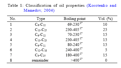
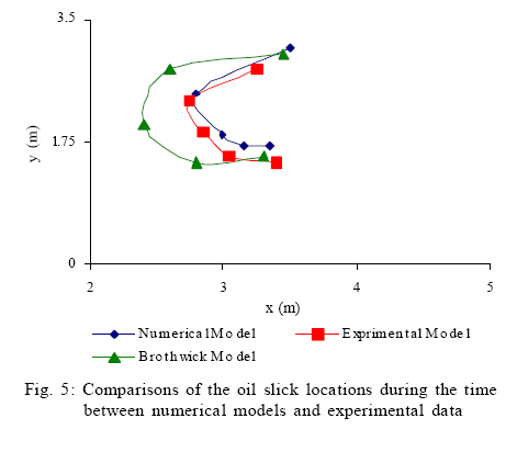
International Journal of Environment Science and Technology, Vol. 7, No. 4, 2010, pp. 771-784 Numerical modeling of two-phase fluid flow and oil slick transport in estuarine water M. Nagheeby;*M. Kolahdoozan Department of Civil and Environmental Engineering, Amirkabir University, Tehran, Iran *Corresponding Author Email: mklhdzan@aut.ac.ir Tel.: +9821 6454 3023; Fax: +9821 6641 4213 Received 18 Jannuary 2010; revised 6 May 2010; accepted 26 June 2010 Code Number: st10076 ABSTRACT: Oil spills is one of the most important hazards in the estuarine and coastal water. In recent decades, engineers try to predict the status of oil slick to manage the pollution spreading. The prediction of oil slick transport is carried out mainly by means of numerical models. In the current study, the development and application of a two-phase fluid flow model to simulate oil transport in the marine environment are presented. Different transport and fate processes are included in the developed model. The model consists of the Lagrangian method for the advection process, the Random Walk technique for horizontal diffusion process and the empirical equations for the fate processes. The major forces for driving oil particles are fluid current, wind speed and turbulent flow. Therefore, the multi-component hydrocarbon method has been included to the developed model in order to predict fate processes. As prediction of particle velocity components is of major importance for oil slick advection, therefore the binomial interpolation procedure has been chosen for the particle velocity components computations. In addition, shoreline boundary condition is included in the developed model to simulate shore response to oil slick transport near the beaches. The results of the model applications are compared with the analytical solutions, experimental measurements and other numerical models cited in literature. Comparisons of different sets of results represent the capability of developed model to predict the oil slick transport. In addition, the developed model is tested for two oil spill cases in the Persian Gulf. Keywords: Advection; Diffusion; Lagrangian model; Mathematical modeling; Oil spill; Particle tracking; Pollution INTRODUCTION Oil spills are the serious environmental hazards which often exhibit long-term impacts. In order to control the damages caused by oil pollution, operational modelling is needed to provide real-time prediction of the transport and fate of the spill. These models can be used in decision making processes to select the most efficient and appropriate solution (Cheng et al., 2000; Li, 2001; Ventikos et al., 2004; Liu and Writz, 2006; Bandyopadhyay and Chattopadhyay, 2007; Tuzkaya and Gulsun, 2008). The oil spill in seawaters has the complex physical, chemical and biological processes which should be considered in numerical modeling (Gallardo and Marui, 2007). The processes are divided into three phases: oil on the surface layer, oil in the water column and oil in the bed layer. In each phase, some processes are of major importance. Furthermore, the mass exchange exists in the interfaces (Patankar and Joseph, 2001; Mossalanejad, 2009). Oil spill models can be developed by either Eulerian or Lagrangian approaches. Using Lagrangian models, the phenomena is mostly represented by a large number of small particles which are advected by fluid velocity at the water surface. Introducing the physical properties of the phenomena based on the particle tracking approach is very complex and needs special attention regarding different aspect of modeling (Nagheeby, 2006). In the Eulerian approach, the mass and momentum equations are applied to the oil slick layer. By comparing these two approaches, it can be concluded that although the Lagrangian approach is more complex, it can well represent the location of oil slick and also predict the oil slick breakage due to the flow pattern (ASCE Task Committee, 1996; Rowshan et al., 2007). Generally, in multiphase problems in which the floating phase does not affect the outside domain, such as the transport of oil in the water, simulations were made based on the Lagrangian approach (Yapa et al., 1999; Yapa and Chen, 2004). Therefore, a Lagrangian discrete particle algorithm is used to simulate the oil slick transport. In the recent decades, many researchers have studied the transport and fate processes of oil spills based on the trajectory method and mass balance approach, i.e. (Yapa et al., 1994; 2002; ASCE Task Committee, 1996; Reed et al., 1999) as reported by Chao et al. 2003. Some well-established models such as OILMAP developed by the Applied Science Associations in 1997, SINTEF developed by Reed in 2000 and GNOME developed by the National Oceanic and Atmospheric Administration (NOAA) in 2001, are being used currently to predict oil transport and distribution in a water body (Chao et al., 2003, Nouri et al., 2008; 2009; Adams et al., 2009). Among these oil spill models, many focus on the surface transport. In this study, a two-dimensional two-phase numerical model is developed to predict the transport and fate of oil slicks, which resulted in the concentration distribution of oil to be on the water surface. Two dimensional governing equations of fluid flow which consist of mass and momentum were solved using the finite difference method on the structured staggered grid system (Falconer, 1976). The resulted algebric equations were solved by the alternating direction implicit (ADI) technique. In addition the wind speed and the coriolis effects were included in the current hydrodynamic model. The transport of the oil slick was predicted by the two dimensional particle tracking approach consisting of the Lagrangian method for the advection processes, the Random Walk technique for the horizontal diffusion process and the empirical equations for the fate processes. Fate processes were simulated using multi-component method in order to consider the oil composition (Table 1). In addition the shoreline response to oil slick transport was also included in the developed model. This study was carried out in Tehran, Polytechnic during 2005-2006 and supported financially by The National Iranian Refining and Distribution Company. MATERIALS AND METHODS Mechanism of physical-chemical interaction of oil spill Two different processes were recognized when oil spilled into the water. The first process dominated the transport of the oil slick due to the coastal currents, which include advection, spreading and turbulent diffusion. The second process was related to the interface interaction of the oil slick with air and water. At oil-air interface, evaporation could be observed, while at the oil-water interface dissolution, emulsification and sedimentation were dominated (Han et al., 2001). Oil spill processes are related to oil properties, hydrodynamic and environmental conditions. When oil is spilled into the seawater, it spreads to form a thin film. The oil slick transports by the advection and turbulent diffusion due to the surface current, waves and wind. Furthermore, the slick spreads due to a balance of forces. From the physical point of view, the transport of oil slick includes the fate processes resulting in a thinner layer of oil on water surface. Finally, when slick comes to a critical thickness, it will be divided into small portions (Koziy and Maderich, 2003). Advection and turbulent diffusion The main processes involved in the transport of oil on the water surface are advection and turbulent diffusion. Advection is mainly due to the wind, surface current and waves (Hussein et al., 2002). The comparison of results obtained from Lagrangian and Eulerian models showed that results obtained from the earlier one are more accurate, especially in the advection process computations (ASCE Task Committee, 1996). In addition, the slick breakage can be predicted by the Lagrangian approach (Shen and Yapa, 1988). The oil slick is introduced by a large number
of particles which move with the surrounding water
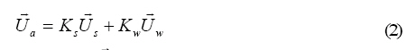
body. Total velocity (
Where, (1) turbulent diffusion. Advective velocity is described as (Al-Rabeh et al., 1989, 1992; Chao et al., 2001, 2003):
Where,
Where, u1,
u2, u3 and u4 are the flow
velocity components, In the other hand, the diffusive velocity (
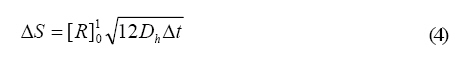
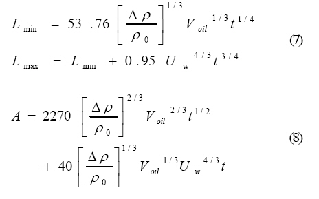
Where, [R]10 is a random number between 0 to 1, and Dh is the horizontal diffusion coefficient. The displacement of the oil slick due to the advection and horizontal diffusion can be calculated by (Al-Rabeh et al., 1989, 1992): Lx(Δt) = Uax Δt + ΔS cos θ Ly(Δt) = Uay Δt + ΔS cos θ (5) Where Lx(Δt) and Ly(Δt) are displacements in the x and y directions, respectively, Uax and Uay are advective velocity components in the x and y directions, respectively and where θ = 2π[Rθ ]10 is a random number between 0 to 1. Finally, the "i" particle at time "n" is transported to the new location at time "n+1" as: X i n+1= X i n + Lx(Δt) Y i n+1= Y i n + Ly(Δt) Where, X and Y are particle coordinates, i is the number of particles, and n and n+1 are the time level. Spreading According to Fay hypothesis, the spreading process is the horizontal expansion of the oil slick due to the counterbalance of mechanical forces including gravity, surface tension, inertia and viscosity (ASCE Task Committee, 1996; Shen and Yapa, 1988). This process dominates the transport at the beginning of oil spilling. Lehr developed a relationship based on Fay's study (Chao et al., 2001, 2003). According to Fay, an elliptical area is covered by the oil slick in which the large diameter is in the direction of wind. Lehr's relationships are as follows (Chao et al., 2001, 2003):
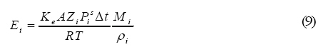
Where, Lmax, Lmin are the length of the major and minor axes of ellipse, respectively (m), A is the area of oil slick (m2),Δρ = ρw - ρ0, ρw , ρ0 are the densities of water and oil, respectively, Voil is the total volume of an oil spill in barrels (1 barrel = 0.1589 m3), Uw is the wind speed in knots and t is time (min). The Lehr formulation is deployed in the developed model. Evaporation Evaporation plays a critical role during the early stages of an oil spill and reduces the oil mass. Oil properties (viscosity and density) are being changed during the evaporation (ASCE Task Committee, 1996). Mackay proposed a mathematical model based on the multi-component theory to estimate the rate of oil evaporation (Chao et al., 2001, 2003) which can be expressed as follows:
Where, Ei is the magnitude of component i lost by the evaporation (m3 ), Ke is the mass transfer coefficient of evaporation (m/s), A is the oil slick area (m2 ), Zi is the amount of oil fraction defined as Zi = Ei /ΣEi (%), Pis is the vapor pressure of component i (atm), Mi is the molecular weight (g/mol), ρi is the density of oil component (gr/m3 ), Δt is the time step (s), R is the gas constant (8.206 × 10⁻⁵ atm.m3 / mol.ºK) and T is the air temperature above the slick (ºK). The estimation of Kd is based on Mackay hypothesis and is defined as (Chao et al., 2001; 2003): Ke = 0.0292Uw 0.78 hs -0.11 Sc -0.67 (10) Where, Uw is the wind velocity (m/s), hs is the oil slick thickness (m) and Sc is the Schmidt number which represents the surface roughness and is assumed to be equal to 2.7 in this study (Khosravi, 1990). Dissolution Some of the oil components, which are subjected to evaporation, can also be dissolved into the water column. The process for simulating dissolution is similar to the evaporation. In this case, a multi-components model based on Mackay hypothesis was deployed as follows (Chao et al., 2001, 2003):
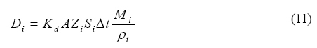
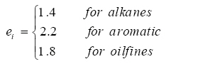
Where, D i is the magnitude of component i lost by dissolution (m3), Kd is the mass transfer coefficient of dissolution (m/s), A is the oil slick area (m2), Zi is the amount of oil fraction (%), Si is the solubility of fraction i, M i is the molecular weight (g/mol), ρi is the density of oil component (g/m3) and Δt is the time step (s). The estimation of is based on Mackay studies and is defined as (Chao et al., 2001, 2003): Kd = 2.36 ×10⁻⁶ ei (12) Where
Vertical dispersion and mixing Dispersion is the break-up of the coherent oil slick into small droplets of varying size, and the spread and diffusion of the droplets in the water column. Smaller droplets will remain suspended in the water whereas the larger ones will rise back to the surface to either reform the oil slick or spread out to form a very thin film of oil. Delvigne and Sweeney proposed a relationship for computing the oil entrainment rate based on oil type, breaking wave energy and particle size as (Chao et al., 2001; 2003): Q (d) = Ken Dba0.57 Scov Fwc dp0.7 Δd (13) Where, dp is the oil particle size (m), Δd is the particle size interval (m), Q (d) is the rate of oil particles entrainment with sizes in an interval Δd around d (Kg/m2s), Ken is a proportionality constant, identified as the entrainment coefficient, Dba is the dissipated breaking wave energy per unit surface area (J/m2), is the fraction of surface area covered by oil (0≤Scov≤1 ), and Fwc is the fraction of sea surface hit by breaking waves per unit time. Dba and Fwc are given as (Chao et al., 2001; 2003): Dba = 0.0034ρw gH2rms (14) Fwc = 0.032 ( Uw - Uwt/Tw (15) Where, pw is water density (Kg/m3), g is the acceleration due to gravity (m/s2), Hrms is the root mean square (rms) wave height (m), Uw is wind speed (m/s), Uwt is the threshold wind speed for a wave breaking (5 m/s) and Tw is the breaking wave period (s). Adsorption of oil by sediment Oil can be trapped in the spaces between sediment particles. This process is divided into two categories:
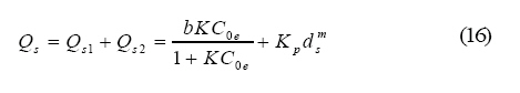
Considering the above two categories, the total absorption can be expressed as (Chao et al., 2001; 2003):
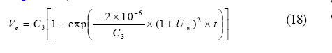
Where, Qs is the total absorption capacity, Coe is oil concentration after absorption balance, ds is the sediment particle diameter and m, Kp, K and b are absorption parameters based on empirical relationships of Chao et al., (2003), which can be shown as: b = 1.96 x 10⁻⁴ ds -0.62 K = -68.31ds + 112.21 Kp = 8.14 x 10⁻⁶ Emulsification Emulsion is the change of mixture of oil and water due to the breaking waves and water turbulence. The formation of emulsions can strongly change the oil properties. The density of the emulsion could be 1.03 times denser than the initial oil density. The first twelve hours of spilling is the most important time with regard to change in density (ASCE task committee, 1996). Viscosity is the most significant parameter as it increases from a few hundred cSt to approximately 50000 cSt. For the emulsion estimation, Mackay's relationship was used in the current study (Shen and Yapa, 1988):
Where Ve is the water content of the emulsion, Uw is the wind speed (m/s), C3 is the constant viscosity equal to 0.7 for heavy oil and 0.25 for light oil, and t is time (s). Change of oil properties Emulsion and evaporation of oil increase the oil viscosity and density. Therefore, these oil properties should be corrected during the oil slick transport. According to Mackay relationships the viscosity of remaining oil and the density of emulsion are as follows: (Wang et al., 2005):
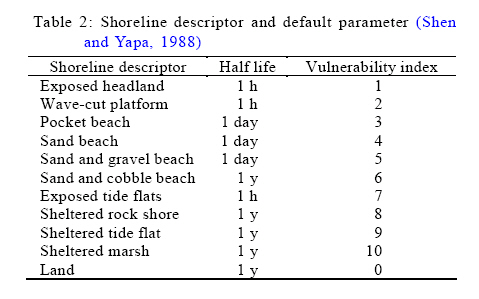
Where, μ is the viscosity of the remaining oil, μ0 is the initial value of the oil viscosity (cP), ρw is the density of water (Kg/m3), is the density of emulsion (Kg/m3), ρc is the initial oil density (Kg/m3), Fe is the evaporation fraction and Ve is the water content of the emulsion. Shoreline boundary condition The interaction of oil and the shoreline is a very complex process both in terms of the environmental and numerical modeling. The damages caused by the Exxon Valdez accident (1989) represent the importance of this phenomenon. Many effective phenomena such as waves, current and wind tend to create coastal response and cause complex problems. Therefore, shorelines should be considered as a boundary condition for oil slick transport (ASCE task committee, 1996). Torgrimson used the half-life method based on exponential decay function (Shen and Yapa, 1988). In this method, a holding capacity was assigned for each type of beach. "Half-life" parameter expresses coastal ability for oil holding. Table 2 shows the half-life and vulnerability index for some beaches (Shen and Yapa, 1988). In this study, based on the half-life method, the volume of oil remaining on the beach is related to its original volume as follows (Shen and Yapa, 1988):
Where,
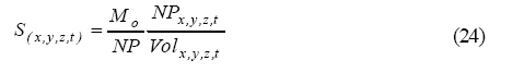
According to Al-Rabeh's studies, the return probability function of the oil particle from shore to the sea can be expressed as (Al-Rabeh et al., 1989, 1992): Pr = 1 − 0.5 t/λ (22) Therefore, those particles which satisfy equation 22, can be returned to the sea. rand (0,1) < Pr (23) Where, Rand (0,1) is a random number in a specified range and Pr is the return probability of the oil to the sea. Concentration conversion According to equation (24), the number of particles is transformed into a concentration at each grid cell (Kang, 1998):
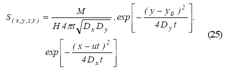
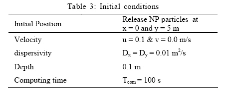
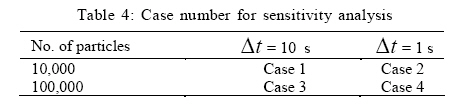
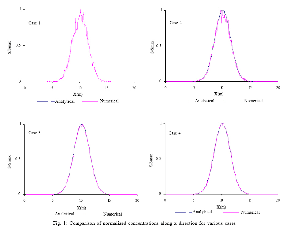
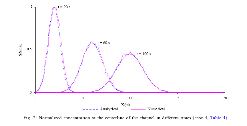
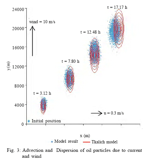
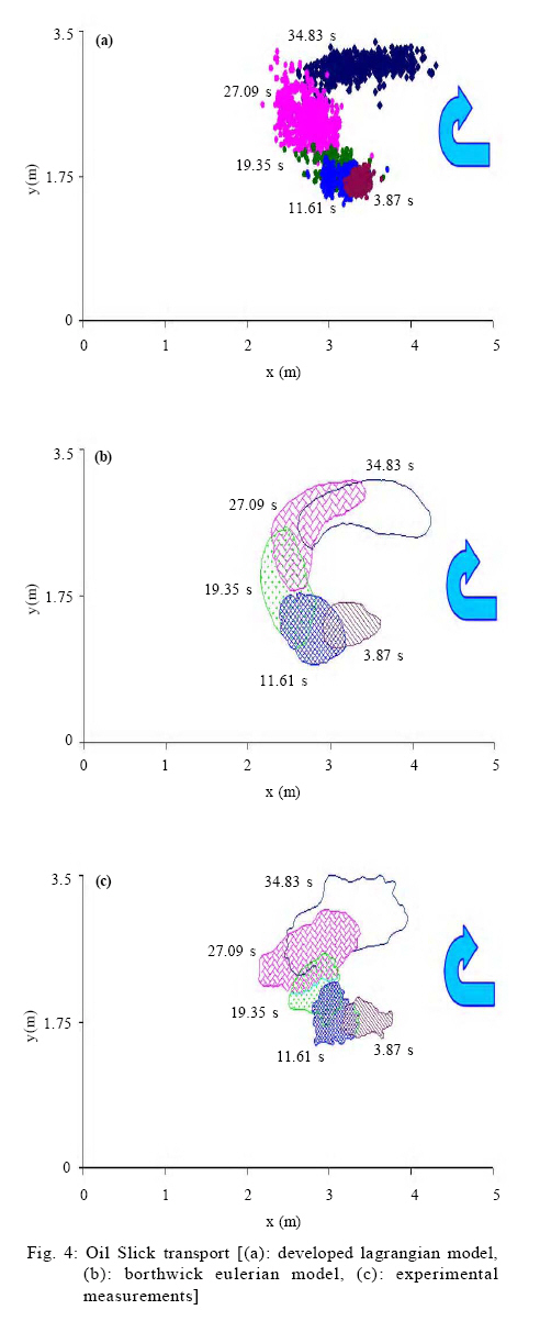
Where, S(x,y,z,t) is the oil particles concentration of a grid cell, Mo is the total mass of oil spilled into the computational domain, NP is the total number of particles in the computational domain, NPx,y,z,t is the total number of particles in a grid cell, and Volx,y,z,t is the volume of a grid cell. Oil spill simulation In order to simulate oil transport in estuarine waters, a two-dimensional multi-phase oil slick transport model was developed in the current study. The model consists of two sub-model namely hydrodynamic and oil slick transport. In each time interval, flow pattern was obtained from the hydrodynamic sub-model (DIVAST). Two dimensional governing equations of fluid flow which consist of mass and momentum conservation were solved using an implicit finite dfference method on the structured staggered grid system. The resulted algebric systems of equations were solved by the ADI technique. After determining the horizontal velocity components at each Eulerian mesh points, the oil transport sub-model was called in order to simulate oil slick transport. In this sub-model, it is assumed that oil slick is produced by individual particles. It is obvious that the number of particles has direct effect on the accuracy of numerical modeling results. The initial condition was introduced in a way that an initial portion of the area under the study is covered by an oil slick. The new location of oil particles was calculated by considering transport and fate processes based on the presented relationships. It is essential to point out that as the oil particles have not major effect on the flow parameters (Chao et al., 2001, 2003), therefore velocity of oil particles is assumed to be the same as velocity of water. In each time step, if the oil particles reach the shoreline, a related calculation was commenced RESULTS AND DISCUSSION Model validation and verification Validation and verification of the numerical model were carried out with three case studies cited in the literature. Results were compared with analytical solutions, laboratory measurements and other numerical model cited in the literature. Open channel flow In this case, a rectangular channel 20 m length and 10 m width is considered. Uniform grid size of 0.1 m is used both in the x and y directions. Unidirectional flow with 0.1 m/s velocity is assumed along the longitudinal axis of the channel. Dispersion coefficient is set to 0.01 m2/s in both x and y directions. The initial position of the particles is y = 5 m. Simulation time was set to 100 seconds (Kang, 1998). Table 3 presents the initial condition for this case study. Different cases were selected for the sensitivity analysis purposes and were summarized in Table 4. Depth, velocity and dispersion coefficient are assumed constant. The surface concentration of oil can be evaluated analytically using advection-diffusion equation (Kang, 1998):
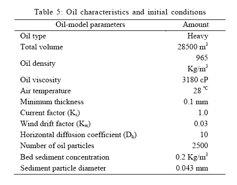
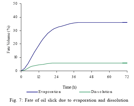
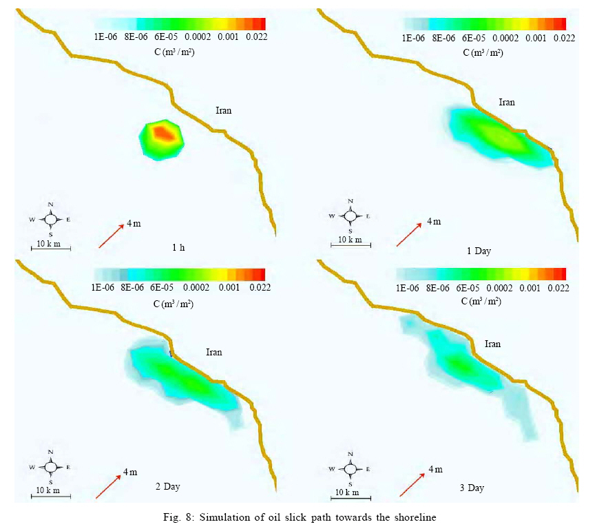
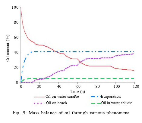
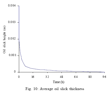
Where M is the total mass of tracer injected at y = 5 m and t = 0, u is the mean velocity, Dx and Dy are the dispersion coefficients in the x and y directions, respectively, H is the depth and t = time (s). Fig. 1 represents the effect of the number of particles and the time step on the accuracy of the results. From Fig. 1, it can be observed that by increasing the number of particles and/or decreasing the time step, more results that are accurate can be achieved. Fig. 1 shows that the combination of 100,000 particles and 1 s time step lead to a more accurate result in this case study. Fig. 2 represents the quantitative simulation results obtained from the numerical and analytical approaches in the centerline of the channel. The accuracy and consistency of numerical prediction in comparison with the analytical computation represent the applicability of the incorporated approaches to the developed numerical model. Oil slick transport due to surface current, wind and turbulent diffusion In this case study, the combination of wind induced and water surface variation currents have been considered to obtain the oil slick trajectory. The total number of particles is set to 5000, which were released at point (400, 800). Total simulation time was set to 24 h with 360-seconds time step. Current velocity components are assumed to be 0.3 and 0.0 m/s for the x and y directions respectively. Wind velocity is 10 m/s constant in the y direction. In addition, dispersion coefficients are set to a constant value of 10 and 2 m2/s for the x and y directions respectively (Tkalich et al., 2003). Numerical model results were compared with an Eulerian model originally developed by Tkalich and Chao in 2001 (Fig. 3) (Chao et al., 2001; Tkalich et al., 2003). The comparison of these two sets of results show that in early stages of the study both models have nearly the same predictions, but after some-time the discrepancy of results between two models can be observed. To find out which one of the above-mentioned approaches is more accurate, a laboratory experimental measurement was chosen which will be presented in the next section. Oil spill in laboratory test To validate the developed numerical model, the laboratory experimental measurements of Borthwick and Joynes (1992) is chosen. These sets of experiments were carried out in the Hydraulic laboratory of the Department of Civil Engineering at the University of Salford, UK. Also, the results of Eulerian numerical model developed by Borthwick is compared with the developed model and the accuracy of Eulerian and Lagrangian approaches are compared. The experimental tank has an overall plan area of 3.50 m × 7.24 m and is elevated 0.7 m above the laboratory floor (Borthwick and Joynes, 1992). Regular waves were produced at one end of the basin by a piston-type paddle driven a 4 hp, 500 rpm variable-speed engine. The maximum plan area of the water surface was restricted to 3.5 m × 5.0 m between the plan-spending beach and paddle generator (Borthwick and Joynes, 1992). A half-periodic sinusoidal lower beach was fabricated, ensuring that the circulation pattern was developed in accordance with the finding of Noda (1974) and da silva Lima (1981) as reported by Borthwick and Joynes (1992). For the experimental study described in this section, the deep water was 0.255 m at the paddle location (Borthwick and Joynes, 1992). Numerical modeling based on the Eulerian approach was carried out by the means of a wire grid with 0.2 m and 0.35 m spacing in the offshore x-direction and long shore y-direction, respectively (Borthwick and Joynes, 1992). During the main test, once steady-state current condition is reached, the oil was spilled from a beaker into the basin at (3.7, 1.4) m and an elevation of no more than 4 cm above the water surface in less than one second. These experimental specifications were selected by trial and error to avoid the spreading of the oil to the side walls during the early stages of the test (Borthwick and Joynes, 1992). Regular waves were generated with the period of 1.29s and offshore deep-water height of 0.098 m (at the paddle) in both numerical models and experimental apparatus. Borthwick has selected a 0.255s time step for his Eulerian numerical model while in the current study a 0.02s was chosen, which corresponds to the courant number less than one. 1000 particles are chosen for numerical modelling purposes while for the flow model a uniform grid spacing of 0.25 m are incorporated. It is essential to point out that the number of particles is case-sensitive, therefore in each case study an appropraite number of particles which is a function of many parameters. physical phenomena, geometry of study area, etc. needs to be found. In terms of Borthwick Eulerian model, a rectangular grid cell with 0.2 m and 0.35 m spacing in the x and y directions respectively have been used, while for the oil slick model, a grid size of 0.05 m has been chosen to achieve a more accurate result (Borthwick and Joynes, 1992). The diffusion coefficients are set to 0.0004 m2/s in both the x and y directions for both Lagrangian and Eulerian models. The oil slick transport is considered through the total computational time of 38.7 s (30 wave periods). The comparison of experimental measurments, Eulerian and Lagrangian model results are shown in Fig. 4. From Fig. 4, it can be concluded that results obtained from developed Lagrangian model are much closer to the measurements in comparison with Borthwick Eulerian model. According to Borthwick, the differences between experimental measurements and numerical model results are due to scale errors and also the diversity of phenomenon parameters, e.g., oil density, surface tension, turbulence eddy sizes, etc. (Borthwick and Joynes, 1992). The comparison of the experimental measurement and modeling results show that from the beginning of the spill up to 11.61 s (9 wave periods), results are in good degree of similarity (Fig. 4). The major role of oil spreading close to the breaker line is the longshore current, which mainly occurred during 15.48 to 23.22 s (12 and 18 wave periods). At 12 wave periods, the physical slick becomes more or less circular. Then, as the slick was advected further alongshore, the rip current began to stretch the slick in the y-direction, resulting in an elliptical shape with the major axis in a double the length of the minor axis (between 18 and 27 wave periods). In contrast, the simulated slick was stretched in the y-direction by the longshore current until it reached the entrance of the rip current (Borthwick and Joynes, 1992). A quantitative comparison of three sets of results is illustrated in Fig. 5. Fig. 5 show that results obtained from the developed model are much closer to the experimental measurements rather than Bothwick Eulerian model results, proving that the Lagrangian approach is more accurate in comparison with Eulerian approach in terms of oil slick transport predictions. Model application Application to Persian Gulf To demonstrate the capability of model in real cases, two virtual oil spill events in Persian Gulf have been chosen. Persian Gulf is one of the major world waterways in terms of commercial and economic activities, specially exporting oil from the region. Approximately 40 % of total oil transports in the world are carried out through this region. The 60 % of total water pollution in the Persian Gulf is due to oil spill. Persian Gulf approximately covers 1000 × 250 km area. The mean water depth is around 35 m and increases near the Hormouz Strait to 100 m. Persian Gulf is connected to Oman Sea and Indian Ocean through the Hormouz Strait (Nagheeby and Kolahdoozan, 2008). According to previous researches in the region, both winds and tidal currents are the most important hydrodynamic phenomena in the region and density and thermal currents are less important (Nagheeby and Kolahdoozan, 2008). To predict the flow pattern in the study area, a two-dimensional horizontal model which is developed originally by Falconer (1976) and then refined by Kolahdoozan (1999) and Kolahdoozan and Falconer (2003) was used. In each time step, flow parameters were calculated by the hydrodynamic module of the model and then these parameters are using in the oil spill sub-model to predict the oil slick trajectory in the study area. Flow pattern in Persian Gulf To prescribe the flow pattern, a rectangular mesh of 2000 m in both x and y directions have been chosen. Open boundary condition was set to water elevation at Hormouz Strait. The no-slip boundary condition was selected for bottom boundaries. According to previous studies in the region, the bed roughness of 400 mm is suitable and is produced calibrated results for flow pattern and water elevation near the Bushehr Bay (Water Research Center, 2000). Oil spill prediction in Persian Gulf Total simulation time is set to 5 days. As a result of cold start for the flow model, the oil spill model starts to predict the oil slick transport at the beginning of the second day. Time step of 72 s are set for both flow and oil spill sub-models. As there is no data available in terms of oil transport in the region for calibration purposes, therefore only the applicability of model is studied. Two oil spill events have been assumed with the 28500 m3 (179260 barrel) volume of oil. Tidal characteristics of 2nd. October 2003 have been considered for modeling purposes. The locations of oil spills were assumed to be approximately in 50 km distance from Bushehr Bay (50º 08" latitude and 29 º 5" longitudes for first event and 50º 80" latitude and 29º 35" longitudes for the second event). A 4 m/s wind speed with the 45-degree blowing at the southeastern direction for first event and northeastern for second one have been assumed. The sand and gravel beach with a half-life of 24 h has been considered. Oil characteristics and initial conditions are summarized in Table 5. Fig. 6 shows the initial location of oil spill and oil slick transport after 3 days for the first event. From Fig. 6, it is observed that the path of oil slick was diverted to the Bushehr Coast. The oil slick area tends to an ellipse with the major diameter in the wind direction in the early stages of modeling. As the flow current in the region is mainly consist of tidal current and wind-induced currents, therefore the direction of ellipse major axis is not exactly in the wind direction. In Fig. 7, the fate of oil slick due to the evaporation and dissolution is presented. Fig. 7 shows that 35 % of oil is evaporated in the first 26 h and only 5 % of oil entered into the water column. Oil slick on the water surface consists of 60 % of the volume, which originally spilled into the water. The oil slick area increased according to Fay's hypothesis and reached the final value. In the second event, the impact of oil slick to the shoreline has been studied. Oil slick parameters are the same as the first event. The oil trajectory and oil concentration are presented in Fig. 8. Fig. 9 demonstrates the oil spill balance in the region at different times. From Fig. 9, it can be concluded that 40 % of oil was evaporated in less than 10 h. The 40 % of oil was absorbed by beach in 120 h and less than 20 % of oi l was remained in the water surface. From Fig. 9 also can be observed that beach absorption is one of the most important phenomena near the coastline. Oil slick thickness is decreased in only 8 h and reaches its final value after 40 h (Fig. 10). Conclusion The Eulerian - Lagrangian model was developed to simulate two-phase fluid flow. This model predicts the oil slick transport, the fate processes and the concentration distribution of oil on the water surface. By coupling a two-dimensional depth averaged hydrodynamic model with the developed oil slick model, oil slick transport can be simulated. Wind effect, as well as water current due to tide is included in the hydrodynamic module. To obtain more accurate simulation results, the binomial interpolation technique was deployed for the prediction of particle velocity components. In addition, the multi-component hydrocarbon method was incorporated to estimate the amount of oil, which die down through the fate processes. Absorption of oil reaches to the shoreline boundary also included in the developed numerical model. The validation and verification of the model were carried out by comparing numerical results with analytical solutions, laboratory measurements test and/or results obtained by numerical models cited in the literature. The comparison of models' results (Borthwick's Eulerian and developed Lagrangian models) show that Lagrangian approach is more accurate than the Eulerian one in terms of oil slick transport predictions. Also, the comparison of model results with analytical solution represents the capability of the model in an idealized case study. Results obtained from above test cases, show that the incorporated approaches in which included in the developed model through this study can lead to the more accurate numerical modeling estimation. In addition, two virtual cases were chosen for the Persian Gulf, demonstrating the potential of the oil spill model prediction in real case studies. ACKNOWLEDGEMENTS The authors wish to acknowledge the National Iranian Refining and Distribution Company for the financial support made for this research study for their support. In addition, the authors thank Dr. Chao (Researcher in the National Center for Computational Hydro Science and Engineering) for his advices. Nomenclature A oil slick area REFERENCES
The following images related to this document are available:Photo images[st10076f6.jpg] [st10076t1.jpg] [st10076f1.jpg] [st10076t5.jpg] [st10076f8.jpg] [st10076t2.jpg] [st10076t3.jpg] [st10076f2.jpg] [st10076f9.jpg] [st10076t4.jpg] [st10076f3.jpg] [st10076f7.jpg] [st10076f10.jpg] [st10076f4.jpg] [st10076f5.jpg] |
| |||||||||


